5 Body condition ~ cytokines

5.1 Libraries

library(vegan)
library(mixOmics)
library(tidyverse)
library(pairwiseAdonis)
library(mlr3)
library(mlr3tuning)
library(rpart)
library(rpart.plot)
library(ggmosaic)
library(ggpubr)
library(EnvStats)
library(gridExtra)
library(grid)
library(PLSDAbatch)

5.2 Data

cyto <- 
  read.csv("Output Files/cleaned_cytokine.csv")
cytobin <- 
  read.csv("Output Files/cleaned_cytokine_bin.csv")

meta <- 
  read.csv("Output Files/metadata_cyto.csv") %>% 
  mutate(iav=gsub("neg", "IAV-", iav),
         iav=gsub("pos", "IAV+", iav))

# Merge cytokine & metadata 
data <- 
  merge(cyto, meta, by="Sample") %>% 
  filter(!is.na(bc_bin)) %>% 
  mutate(bc_bin = factor(bc_bin, levels=c("Poor", "Average", "Robust")))

databin <- 
  merge(cytobin, meta, by="Sample") %>% 
  filter(!is.na(bc_bin)) %>% 
  mutate(bc_bin = factor(bc_bin, levels=c("Poor", "Average", "Robust")))

5.3 Body Condition Range & Bins

quant <- quantile(meta$bodcond, na.rm=TRUE)

ggplot(meta, aes(x=bodcond)) +
  geom_histogram(bins=10, color="black", fill="gray80") +
  labs(x="Body Condition Index", y="Frequency") +
  geom_vline(xintercept=c(quant[2], quant[3], quant[4]), colour="red", linewidth=1) +
  theme_classic()

## Warning: Removed 8 rows containing non-finite outside the
## scale range (`stat_bin()`).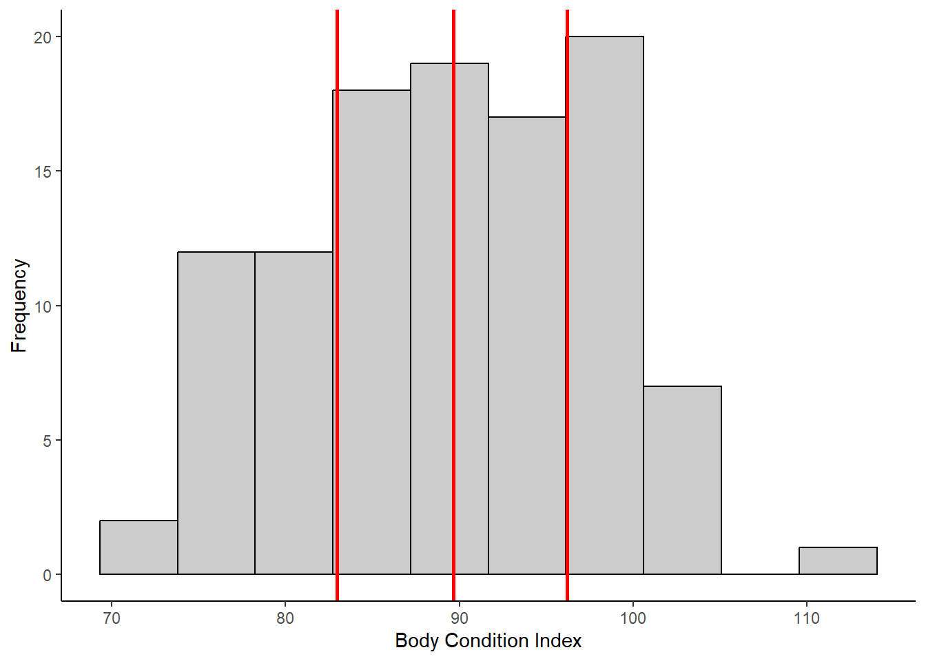

5.4 PERMANOVA

5.4.1 Cytokine Presence/Absence

5.4.1.1 Create similarity matrix (Sorensen)

Dissimilarity = 1-Sorensen

databin_dist <- 
  databin %>% 
  select(2:10) %>% 
  betadiver(., method=11)

plot((1-databin_dist))

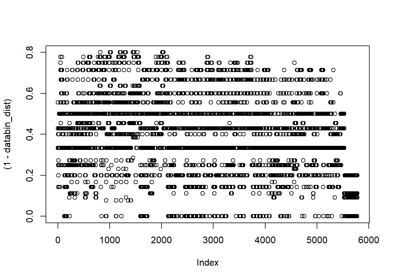
# Dissimilarity summary stats
mean(1-databin_dist); min(1-databin_dist); max(1-databin_dist); median(1-databin_dist)

## [1] 0.3968242

## [1] 0

## [1] 0.8

## [1] 0.4

5.4.1.2 Run PERMANOVA

Use restricted permutation test - data are not exchangeable between analysis years so permute within groups defined by strata.
** Not sig

# define permutations & strata
permute_databin <- 
  how(plots=Plots(strata=databin$analysis.year, type="none"), nperm=4999)

# run permanova
adonis2((1-databin_dist) ~ bc_bin, 
        data=databin,
        permutations=permute_databin)

## Permutation test for adonis under reduced model
## Plots: databin$analysis.year, plot permutation: none
## Permutation: free
## Number of permutations: 4999
## 
## adonis2(formula = (1 - databin_dist) ~ bc_bin, data = databin, permutations = permute_databin)
##           Df SumOfSqs      R2      F Pr(>F)
## Model      2   0.3617 0.03498 1.9032 0.2134
## Residual 105   9.9764 0.96502              
## Total    107  10.3381 1.00000

5.4.1.3 Homogeneity of group dispersions

** Robust vs Poor & Robust vs Average

disper <- 
  betadisper((1-databin_dist), group=databin$bc_bin, type="centroid")

## Warning in betadisper((1 - databin_dist), group = databin$bc_bin, type =
## "centroid"): some squared distances are negative and changed to zero

disper

## 
##  Homogeneity of multivariate dispersions
## 
## Call: betadisper(d = (1 - databin_dist), group = databin$bc_bin, type =
## "centroid")
## 
## No. of Positive Eigenvalues: 8
## No. of Negative Eigenvalues: 35
## 
## Average distance to centroid:
##    Poor Average  Robust 
##  0.3097  0.3086  0.2086 
## 
## Eigenvalues for PCoA axes:
## (Showing 8 of 43 eigenvalues)
##  PCoA1  PCoA2  PCoA3  PCoA4  PCoA5  PCoA6  PCoA7  PCoA8 
## 5.6391 2.8835 2.2162 1.6917 1.5373 0.7135 0.5030 0.3558

anova(disper)

## Analysis of Variance Table
## 
## Response: Distances
##            Df  Sum Sq  Mean Sq F value    Pr(>F)    
## Groups      2 0.19364 0.096822  10.554 6.657e-05 ***
## Residuals 105 0.96323 0.009174                      
## ---
## Signif. codes:  0 '***' 0.001 '**' 0.01 '*' 0.05 '.' 0.1 ' ' 1

TukeyHSD(disper)

##   Tukey multiple comparisons of means
##     95% family-wise confidence level
## 
## Fit: aov(formula = distances ~ group, data = df)
## 
## $group
##                        diff         lwr         upr     p adj
## Average-Poor   -0.001129045 -0.05279805  0.05053996 0.9985132
## Robust-Poor    -0.101094275 -0.16230348 -0.03988507 0.0004504
## Robust-Average -0.099965230 -0.15538277 -0.04454769 0.0001180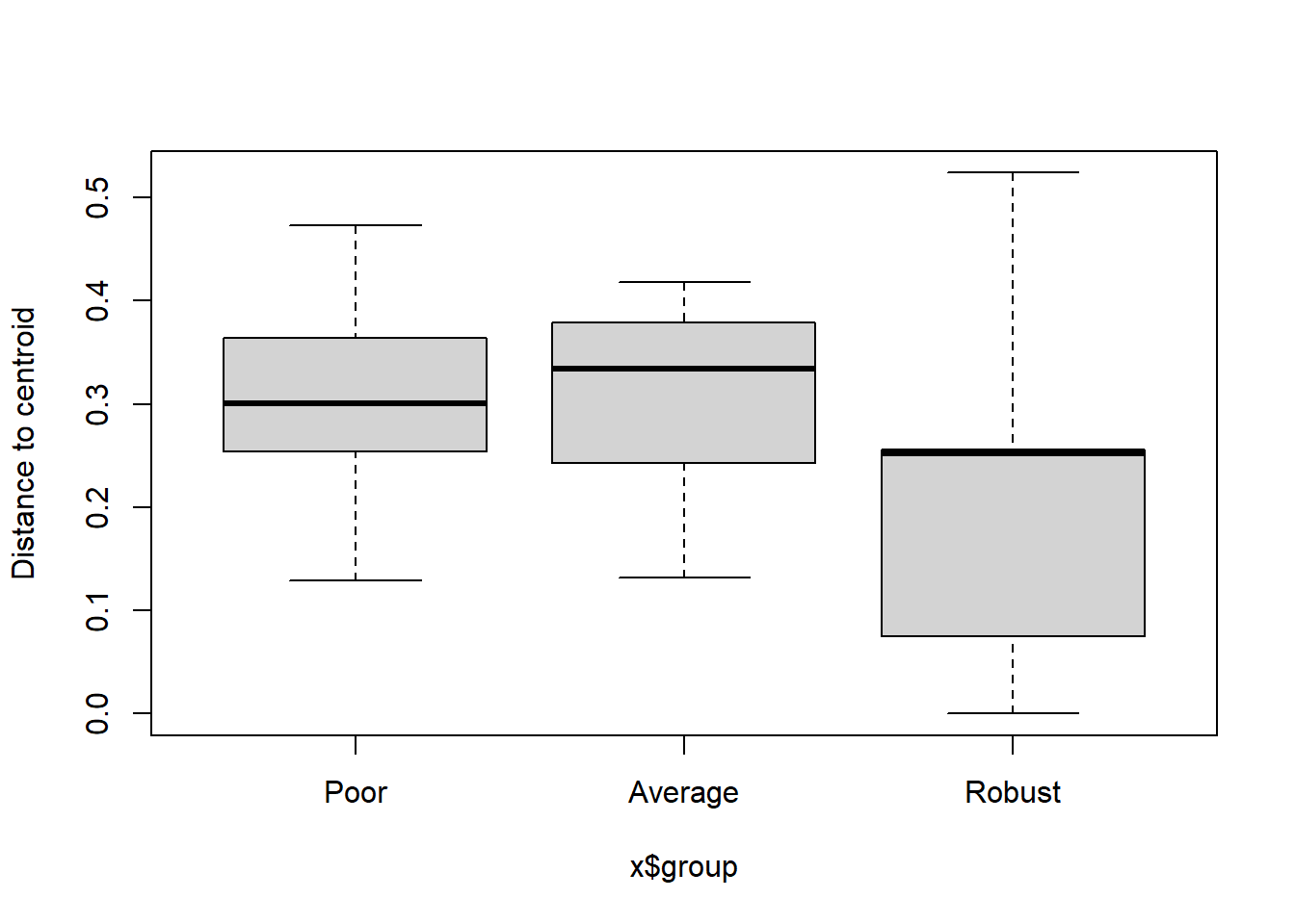

boxplot(disper)

5.4.1.4 Visualization

Principal Coordinates Analysis

# Use 1 - Sorensen's for dissimilarity 
databin_pco <- cmdscale((1-databin_dist), eig=TRUE)

plot(databin_pco$points, type="n", 
     cex.lab=1.5, cex.axis=1.1, cex.sub=1.1)
ordiellipse(ord = databin_pco, 
            groups = factor(data$bc_bin), 
            display = "sites", 
            col = c("deepskyblue", "grey", "darkseagreen"),
            lwd = 2,
            label = TRUE)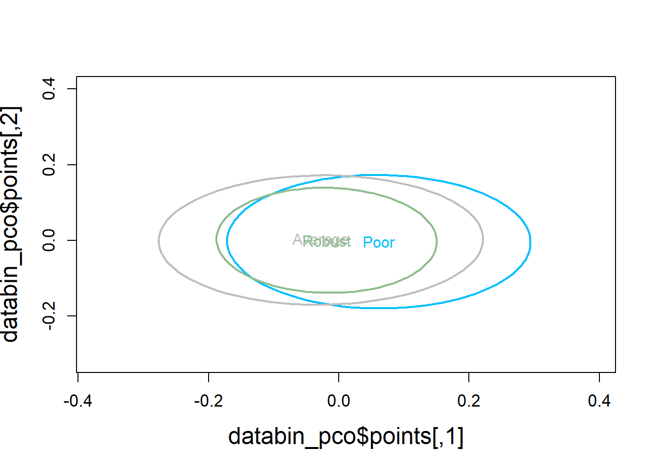

plot(databin_pco$points, type="n", 
     cex.lab=1.5, cex.axis=1.1, cex.sub=1.1)
ordispider(ord = databin_pco,
           groups = factor(data$bc_bin),
           display = "sites",
           col = c("deepskyblue", "grey", "darkseagreen"),
           lwd=2,
           label=TRUE)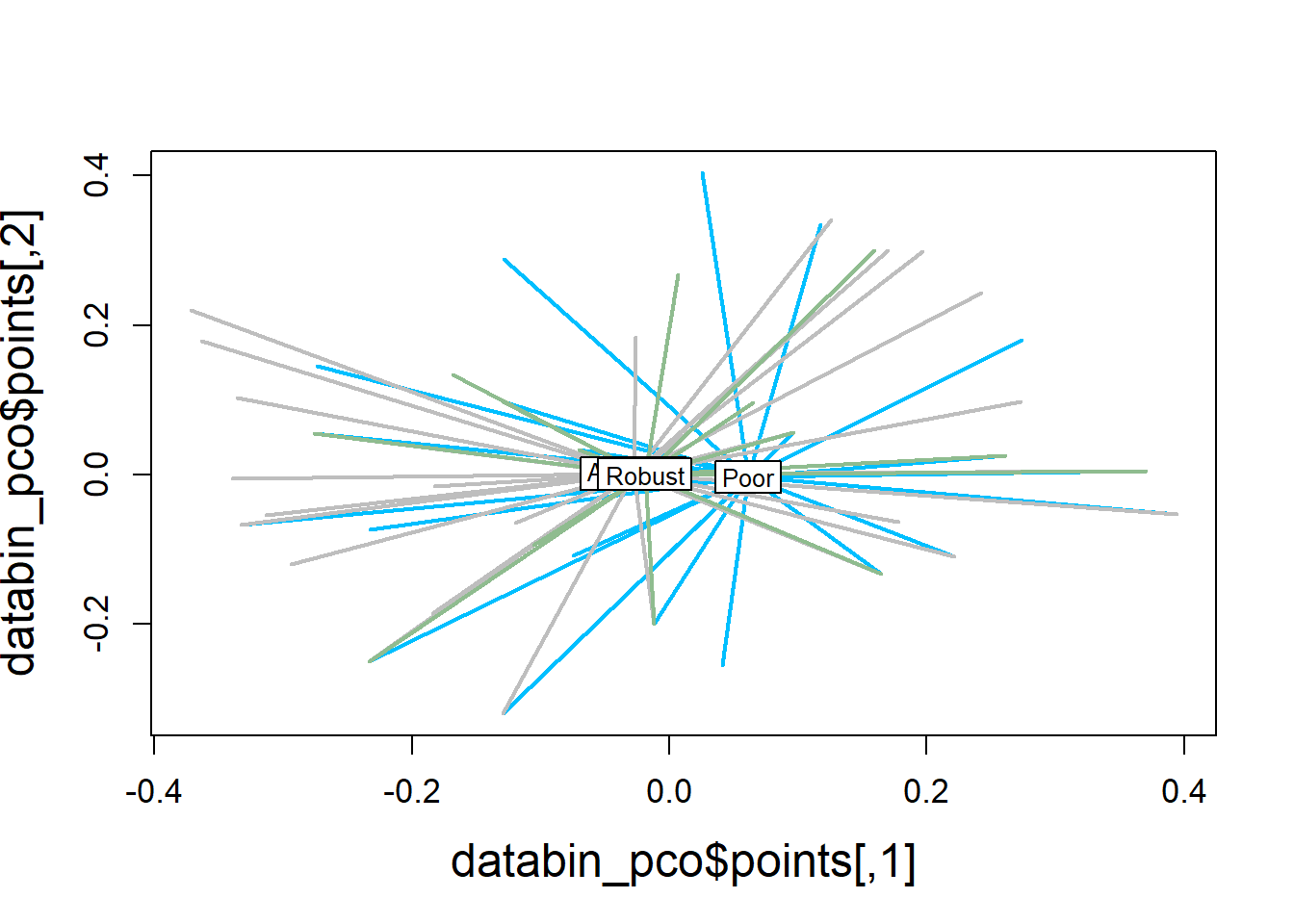

5.4.2 Cytokine Concentration

5.4.2.1 Dissimilarity matrix

data_dist <-
  data %>% 
  select(2:10) %>% 
  vegdist(., method="bray")

5.4.2.2 Run PERMANOVA

** Not sig

# define permutations & strata
permute_data <- how(plots=Plots(strata=data$analysis.year, type="none"), nperm=4999)

# run permanova
adonis2(data_dist ~ bc_bin, 
        data=data,
        permutations=permute_data)

## Permutation test for adonis under reduced model
## Plots: data$analysis.year, plot permutation: none
## Permutation: free
## Number of permutations: 4999
## 
## adonis2(formula = data_dist ~ bc_bin, data = data, permutations = permute_data)
##           Df SumOfSqs      R2      F Pr(>F)
## Model      2   0.3491 0.01973 1.0565 0.5202
## Residual 105  17.3505 0.98027              
## Total    107  17.6997 1.00000

5.4.2.3 Homogeneity of group dispersions

** Not sig

disper <- 
  betadisper(data_dist, group=data$bc_bin, type="centroid")

anova(disper)

## Analysis of Variance Table
## 
## Response: Distances
##            Df  Sum Sq  Mean Sq F value Pr(>F)
## Groups      2 0.02781 0.013903  0.5397 0.5845
## Residuals 105 2.70504 0.025762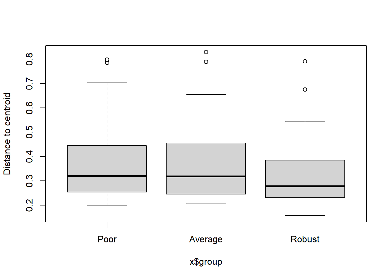

boxplot(disper)

5.4.2.4 Visualization

# Use Bray-Curtis dissimilarity matrix
data_pco <- cmdscale(data_dist, eig=TRUE)

plot(data_pco$points, type="n", 
     cex.lab=1.5, cex.axis=1.1, cex.sub=1.1)
ordiellipse(ord = data_pco, 
            groups = factor(data$bc_bin), 
            display = "sites", 
            col = c("deepskyblue", "grey", "darkseagreen"),
            lwd = 2,
            label = TRUE)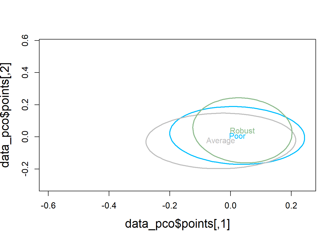

plot(data_pco$points, type="n", 
     cex.lab=1.5, cex.axis=1.1, cex.sub=1.1)
ordispider(ord = data_pco,
           groups = factor(data$bc_bin),
           display = "sites",
           col = c("deepskyblue", "grey", "darkseagreen"),
           lwd=2,
           label=TRUE)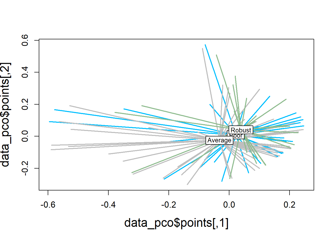

5.5 PLS-DA

5.5.1 Data

pls_x <-
  data[,1:10]  %>% 
  column_to_rownames(var = "Sample")

pls_y <- 
  data %>% 
  select(Sample, bc_bin, analysis.year) %>% 
  column_to_rownames(var = "Sample") %>% 
  mutate_all(as.factor)

5.5.2 Transform data

CLR = Centered log-ratio transformation

pls_x_clr <- 
  logratio.transfo(X = pls_x, logratio = 'CLR', offset = 0.01)

class(pls_x_clr) = 'matrix'

5.5.3 Detect batch effects

Reference: https://evayiwenwang.github.io/PLSDAbatch_workflow/

pca_before <- 
  mixOmics::pca(pls_x_clr, scale=TRUE)

plotIndiv(pca_before, 
          group=data$analysis.year,
          pch=20,
          legend = TRUE, legend.title = "Analysis Year",
          title = "Before Batch Correction",
          ellipse = TRUE, ellipse.level=0.95)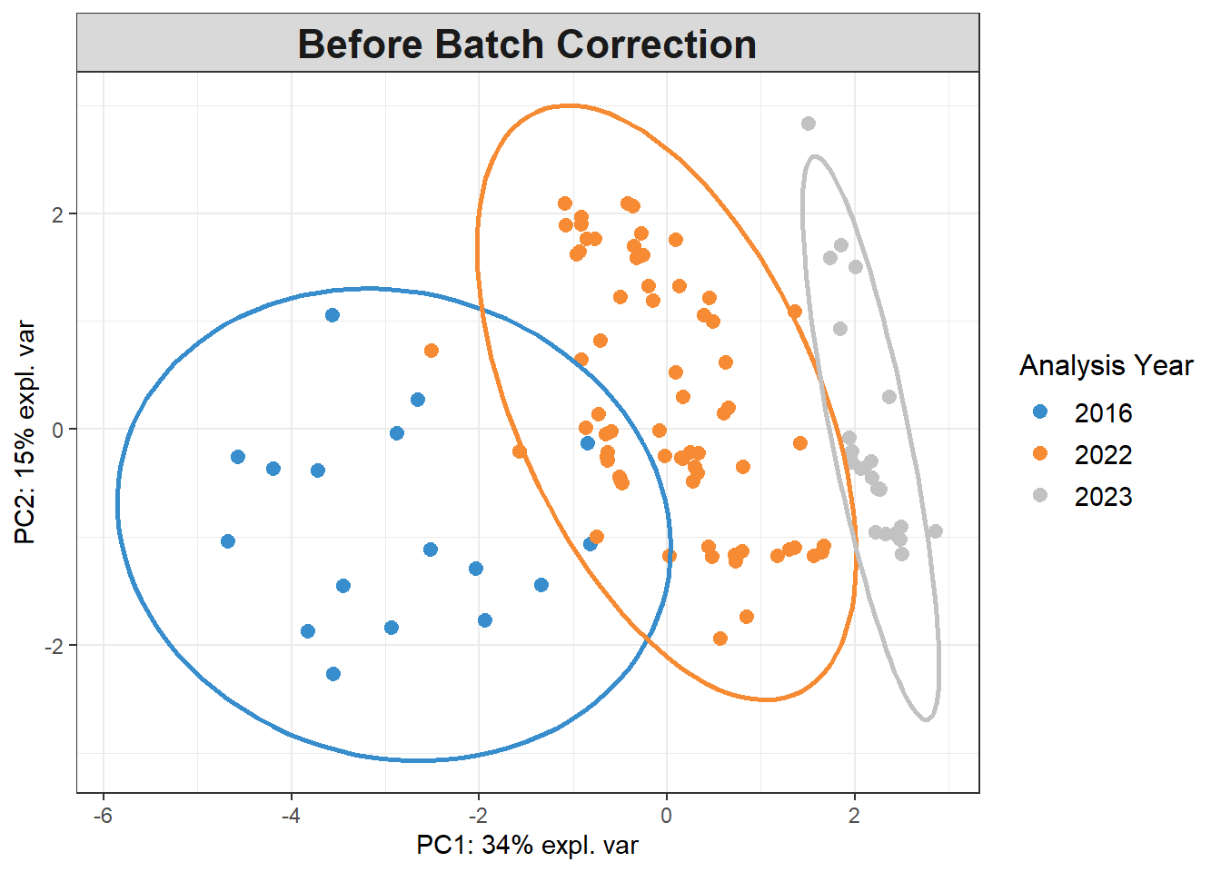

Scatter_Density(object = pca_before,
                batch = pls_y$analysis.year,
                trt = pls_y$bc_bin,
                trt.legend.title = "Body Condition",
                color.set = c("#9d9d9d","#008ba2","black"))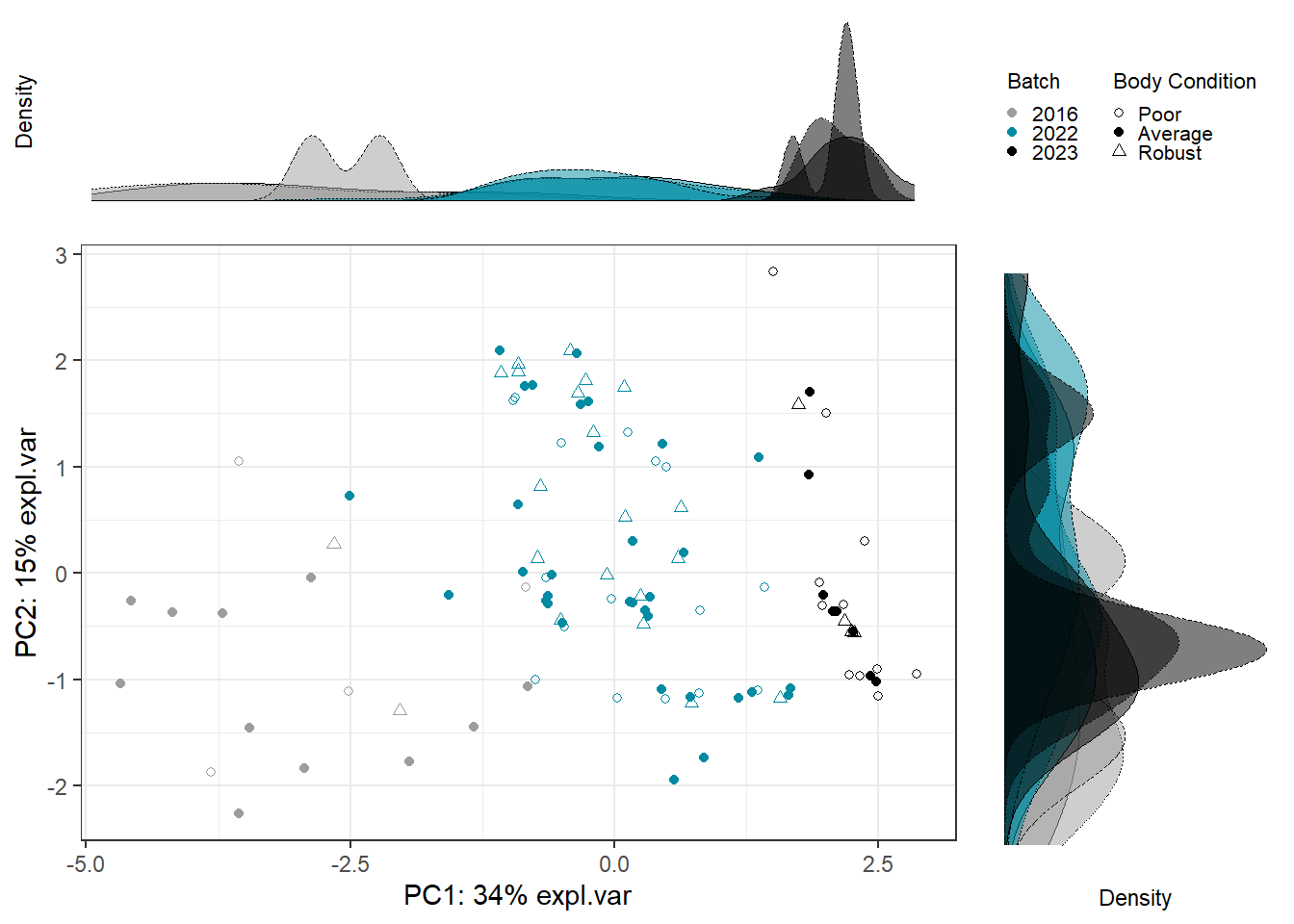

5.5.3.1 Estimate # variable components

Use PLSDA from mixOmics with only treatment to choose number of treatment components to preserve.
Number = that explains 100% of variance in outcome matrix Y.

trt_comp <- 
  plsda(X = pls_x_clr,
        Y = pls_y$bc_bin, 
        ncomp=9)

trt_comp$prop_expl_var

## $X
##      comp1      comp2      comp3      comp4      comp5      comp6      comp7 
## 0.31738239 0.12863676 0.12466645 0.09089348 0.06328953 0.06339432 0.12655617 
##      comp8      comp9 
## 0.08518090 0.19863216 
## 
## $Y
##     comp1     comp2     comp3     comp4     comp5     comp6     comp7     comp8 
## 0.5350530 0.4589453 0.4660231 0.3818196 0.4724626 0.3658912 0.3766012 0.5099951 
##     comp9 
## 0.3803967

sum(trt_comp$prop_expl_var$Y[seq_len(3)]) # preserve 3 comp

## [1] 1.460021

5.5.3.2 Estimate # batch components

Use PLSDA_batch with both treatment and batch to estimate optimal number of batch components to remove.
For ncomp.trt, use # components found above. Samples are not balanced across batches x treatment, using balance = FALSE.
Choose # that explains 100% variance in outcome matrix Y.

batch_comp <- 
  PLSDA_batch(X = pls_x_clr,
              Y = pls_y$bc_bin,
              Y.bat = pls_y$analysis.year,
              balance = FALSE,
              ncomp.trt = 3, ncomp.bat = 9)

batch_comp$explained_variance.bat

## $X
##      comp1      comp2      comp3      comp4      comp5      comp6      comp7 
## 0.32330102 0.27932320 0.19722592 0.08872241 0.11142745 0.01222439 0.05790729 
##      comp8      comp9 
## 0.23005690 0.06316262 
## 
## $Y
##      comp1      comp2      comp3      comp4      comp5      comp6      comp7 
## 0.50837607 0.46461813 0.02700579 0.47992928 0.26376781 0.15443827 0.46656474 
##      comp8      comp9 
## 0.19928134 0.22996614

sum(batch_comp$explained_variance.bat$Y[seq_len(3)]) # preserve 3 comp

## [1] 1

5.5.3.3 Correct for batch effects

Use optimal number of components determined above.
Treatment = 3, Batch = 3

plsda_batch <-
  PLSDA_batch(X = pls_x_clr,
              Y = pls_y$bc_bin,
              Y.bat = pls_y$analysis.year,
              balance = FALSE,
              ncomp.trt = 3, ncomp.bat = 3)

data_batch_matrix <-
  plsda_batch$X.nobatch
  

data_batch_df <- 
  data_batch_matrix %>% 
  data.frame() %>% 
  mutate(bc_bin = pls_y$bc_bin)

write.csv(data_batch_df, "Output Files/batchcorrected_bodycondition.csv")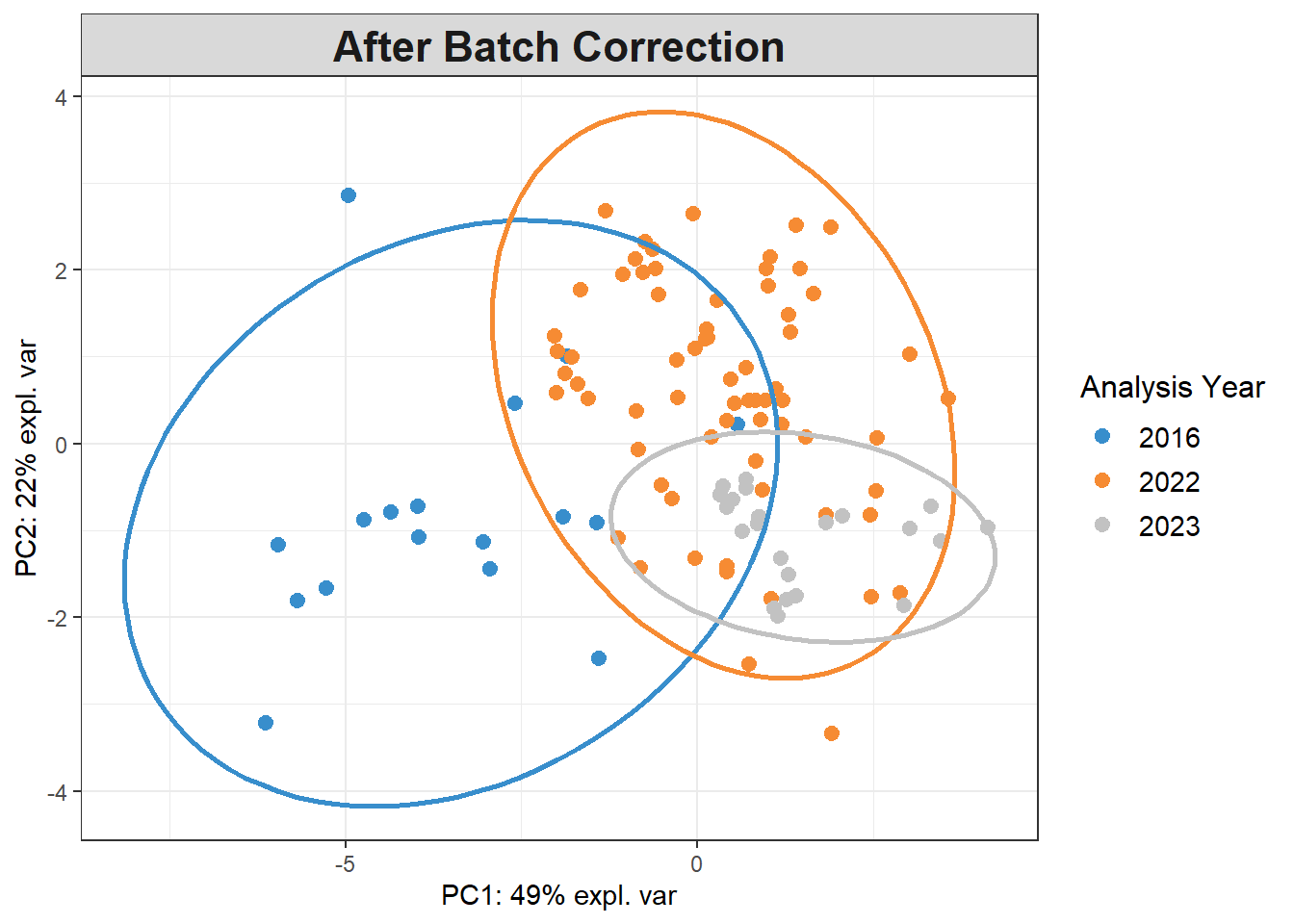

5.5.3.4 Assessing batch correction

after_batch <- 
  mixOmics::pca(data_batch_matrix, scale=TRUE)

plotIndiv(after_batch, 
          group=pls_y$analysis.year,
          pch=20, 
          legend = TRUE, legend.title = "Analysis Year",
          title = "After Batch Correction",
          ellipse = TRUE, ellipse.level = 0.95)

5.5.4 PLSDA on Batch-Corrected Data

plsda_model <- 
  plsda(data_batch_matrix,
        pls_y$bc_bin,
        scale=TRUE)

plotIndiv(plsda_model,
          group=pls_y$bc_bin,
          pch=20, 
          legend = TRUE, legend.title = "Body Condition",
          ellipse = TRUE, ellipse.level = 0.95)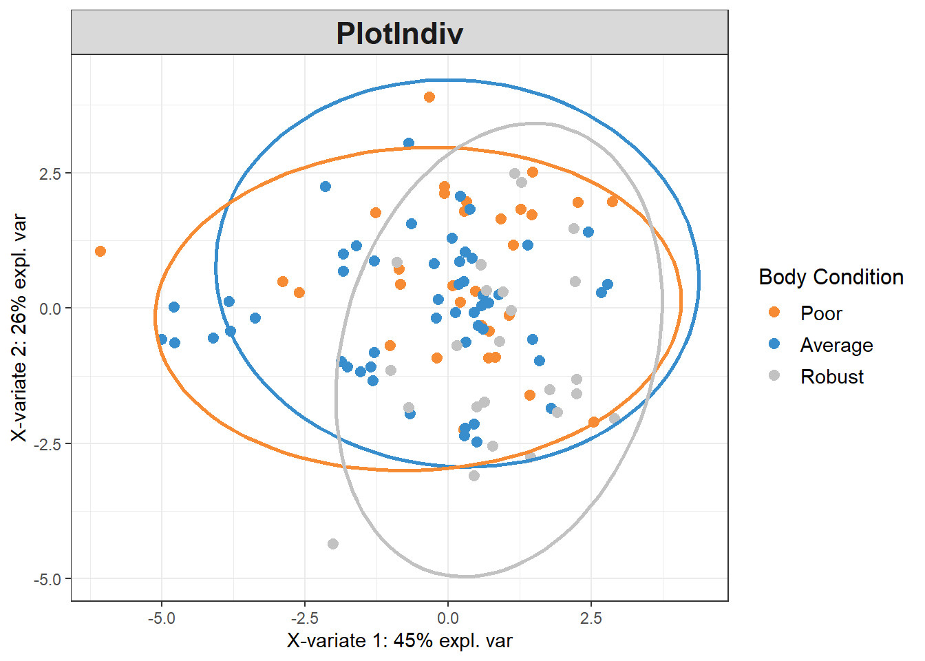

5.5.5 Visualization

5.5.5.1 Set x and y axis labels

labelx <- 
  paste("X-variate 1: ", 
        round(abs(plsda_model$prop_expl_var$X[1]*100), digits=0),
        "% expl. var",
        sep="")

labely <- 
  paste("X-variate 2: ", 
        round(abs(plsda_model$prop_expl_var$X[2]*100), digits=0),
        "% expl. var",
        sep="")

5.5.5.2 Create plot data frame

plsda_ggplot <- 
  data.frame(x = plsda_model$variates$X[,1], 
             y = plsda_model$variates$X[,2],
             bc_bin = plsda_model$Y)

5.5.5.3 Plot

bc_plsda_ggplot <- 
  ggplot(plsda_ggplot, 
         aes(x=x, 
             y=y,
             col=bc_bin)) +
  geom_point() +
  stat_ellipse() +
  labs(x=labelx,
       y = labely,
       name="Body Condition") +
  scale_color_manual("Body Condition",
                     values=c("#9d9d9d","#008ba2", "black")) +
  theme_bw() +
  theme(panel.grid = element_blank())

bc_plsda_ggplot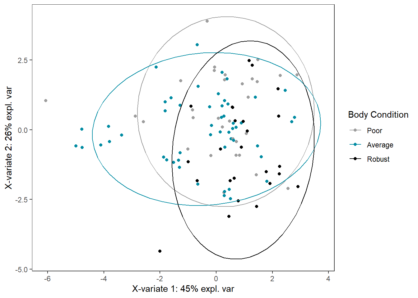

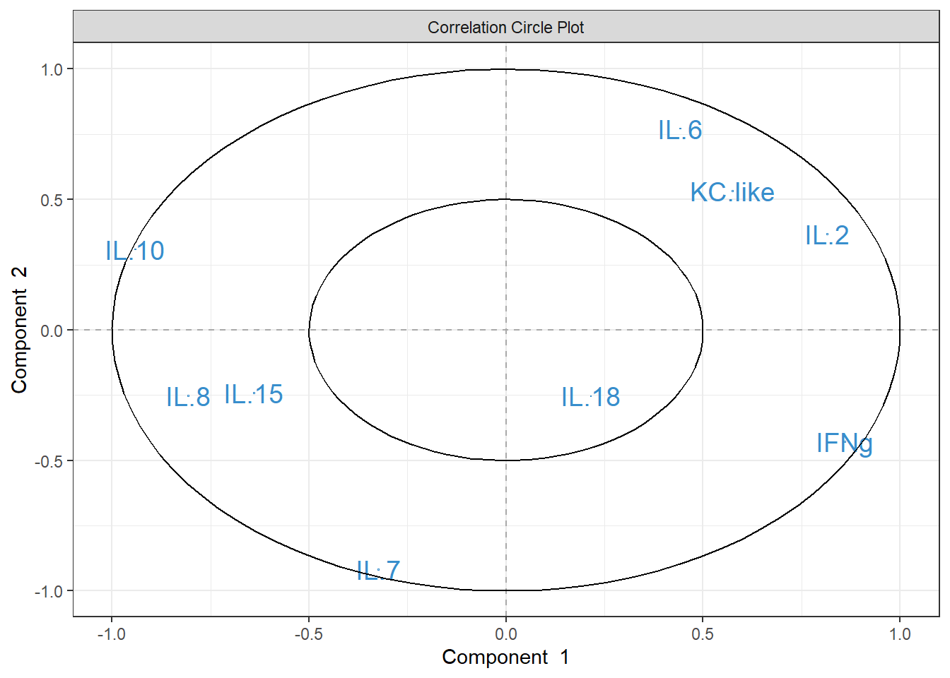
# Presentation
bc_plsda_pres <- 
  bc_plsda_ggplot + 
  labs(title = "Body Condition") +
  theme(legend.position = "right",
        text = element_text(size = 18))
ggsave("Figures/bodycondition_presentation.jpeg", bc_plsda_pres,
       width = 8, height = 6, units = "in")

5.5.6 Cytokine Contributions

plsda_loadings <- 
  plsda_model$loadings$X %>% 
  data.frame() %>% 
  select(1:2) %>% 
  arrange(comp1)
plsda_loadings

##               comp1       comp2
## IL.10   -0.57785153  0.20015962
## IL.8    -0.39137488 -0.21299820
## IL.15   -0.31001015 -0.11902472
## IL.18    0.04164036 -0.05833014
## IL.2     0.08230983  0.24591548
## IL.7     0.15436553 -0.56838363
## KC.like  0.23766248  0.22575495
## IL.6     0.27899879  0.60357885
## IFNg     0.50014567 -0.31335523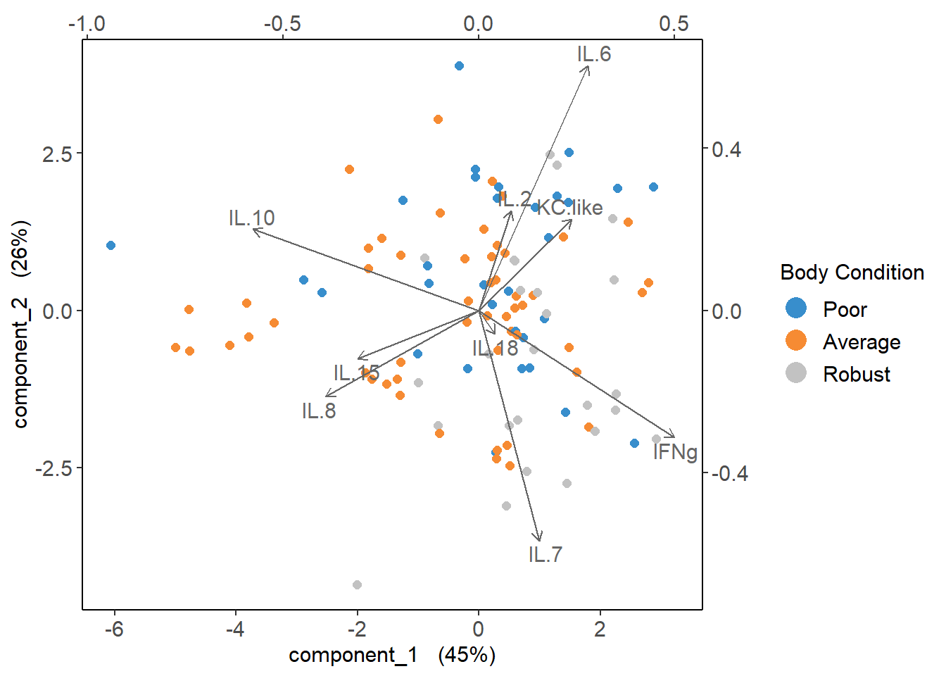

biplot(plsda_model, ind.names=FALSE, legend.title="Body Condition")

plotVar(plsda_model)

5.6 CART

Cytokine Importance ### Prepare data

data_cart <- 
  data %>% 
  select(2:10, bc_bin) %>% 
  mutate(bc_bin=factor(bc_bin, levels=c("Poor", "Average", "Robust")))

5.6.1 Cross Validation

See reference: https://mlr3book.mlr-org.com/

# Creating task and learner
task <- as_task_classif(bc_bin ~ ., 
                        data = data_cart)

task <- task$set_col_roles(cols="bc_bin",
                           add_to="stratum")

# Minimum body condition group size = 25
learner <- lrn("classif.rpart",
               predict_type = "prob",
               maxdepth = to_tune(2, 5),
               minbucket = to_tune(1, 25),
               minsplit = to_tune(1, 30)
               )

# Define tuning instance - info ~ tuning process
instance <- ti(task = task,
               learner = learner,
               resampling = rsmp("cv", folds = 10),
               measures = msr("classif.ce"),
               terminator = trm("none")
               )

# Define how to tune the model
tuner <- tnr("grid_search", 
             batch_size = 10
             )

# Trigger the tuning process
#tuner$optimize(instance)
 
# optimal values: 
  # maxdepth = 4
  # minbucket = 3
  # minsplit = 20
  # classif.ce = 0.5058159

5.6.2 Run CART

cart_model <- rpart(formula = bc_bin ~ .,
                    data = data_cart,
                    method = "class",
                    maxdepth = 4,
                    minbucket = 3,
                    minsplit = 20)

# plot optimized tree
rpart.plot(cart_model)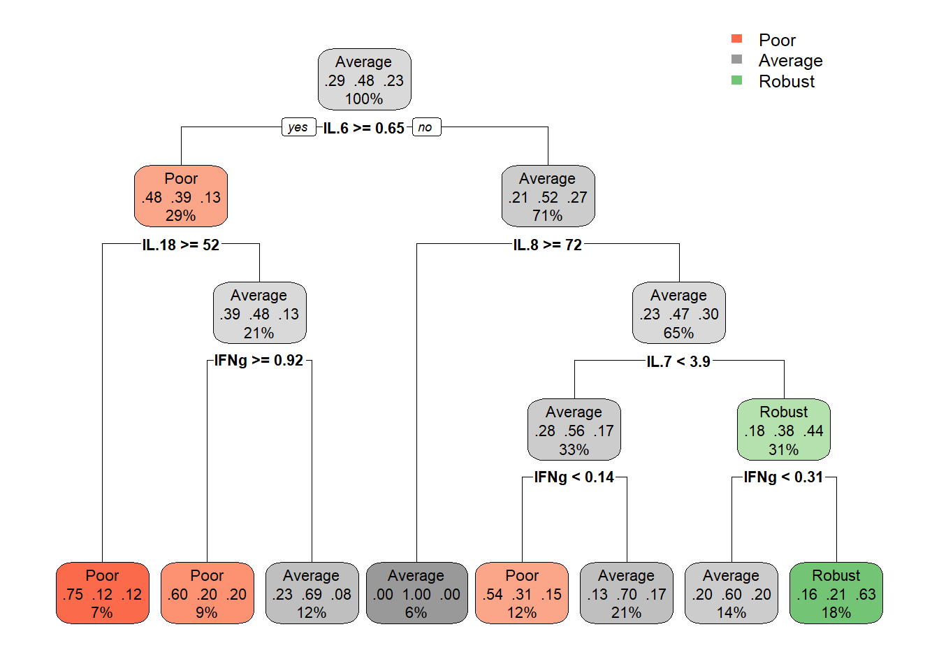

cart_model$variable.importance 

##      IFNg     IL.18      IL.7      IL.6   KC.like      IL.8      IL.2     IL.10 
## 8.2395276 4.0308782 3.2719627 3.1615886 2.9903868 2.6831169 2.2012003 1.1462952 
##     IL.15 
## 0.7364543

# IFNg is most important cytokine

5.6.3 Plot

5.6.3.1 Variable Importance

varimp <- 
  data.frame(imp=cart_model$variable.importance) %>% 
  rownames_to_column() %>% 
  rename("variable" = rowname) %>% 
  arrange(imp) %>%
  mutate(variable=gsub("\\.","-",variable),
         variable = forcats::fct_inorder(variable))

varimp_plot <- 
  ggplot(varimp) + 
  geom_segment(aes(x = variable, 
                   y = 0, 
                   xend = variable, 
                   yend = imp), 
               linewidth = 0.5, 
               alpha = 0.7) +
  geom_point(aes(x = variable, 
                 y = imp), 
             size = 1, 
             show.legend = F,
             col="black") +
  labs(x="Cytokine", 
       y="Variable Importance") +
  coord_flip() +
  theme_classic() +
  theme(text=element_text(size=10, color="black"))
varimp_plot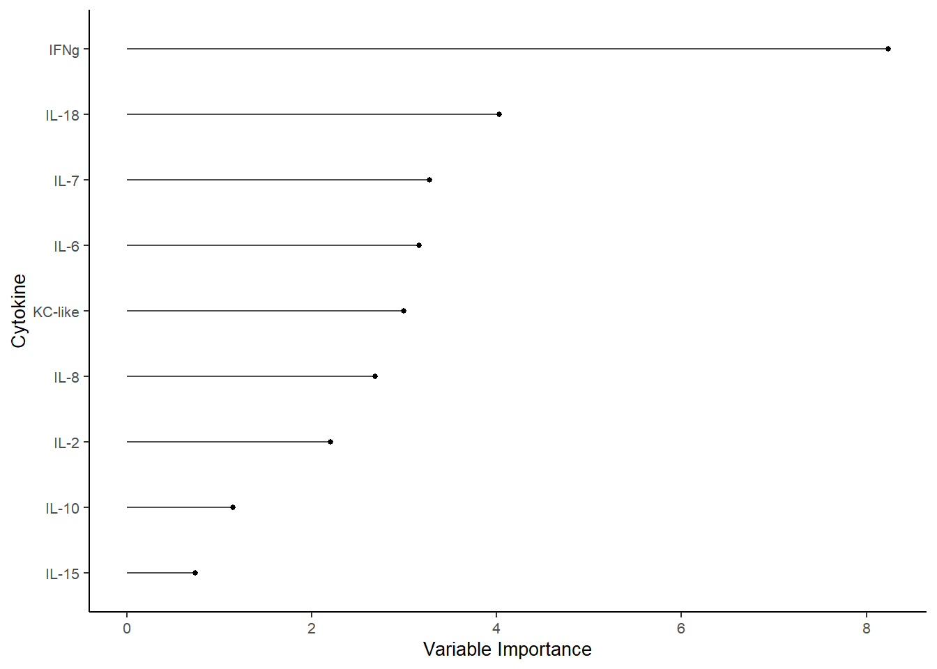

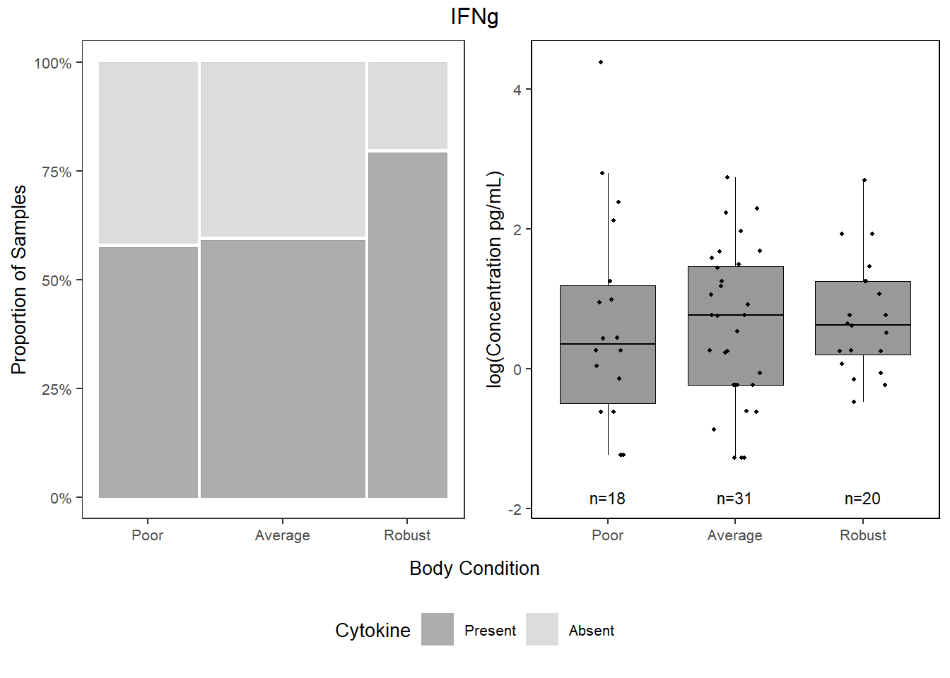
5.6.3.2 Proportions

prop.table(table(databin$bc_bin, databin$IFNg), margin=1)*100

##          
##                  0        1
##   Poor    41.93548 58.06452
##   Average 40.38462 59.61538
##   Robust  20.00000 80.00000

ifng_prop <- 
  databin %>% 
  mutate(IFNg=gsub("1", "Present", IFNg),
         IFNg=gsub("0", "Absent", IFNg),
         IFNg=factor(IFNg, levels=c("Present", "Absent"))) %>%
  ggplot(data=.) +
  geom_mosaic(aes(x=product(IFNg, bc_bin), fill=IFNg)) +
  scale_fill_manual(values=c("Present"="gray60", "Absent"="lightgray"),
                    name="Cytokine") +
  scale_y_continuous(labels = scales::percent) +
  labs(y="Proportion of Samples") +
  theme_bw() +
  theme(panel.grid.major = element_blank(), 
        panel.grid.minor = element_blank(),
        axis.title.x = element_blank(),
        legend.position="bottom",
        text = element_text(size=10),
        plot.title = element_text(hjust = 0.5))

cyto_leg <- 
  get_legend(ifng_prop)

ifng_prop <-
  ifng_prop +
  theme(legend.position="none")

5.6.3.3 Concentration

ifng <-
  data %>% 
  select(bc_bin, IFNg) %>% 
  filter(!IFNg==0) %>% 
  ggplot(., aes(x=bc_bin, y=log(IFNg))) +
  geom_boxplot(color="black", fill="gray60", lwd=0.25,
               outliers=FALSE) +
  geom_point(size=0.75, position=position_jitter(width=0.2)) +
  labs(x=NULL, y="log(Concentration pg/mL)") +
  stat_n_text(size=3) +
  theme_classic() +
  theme(text = element_text(size=10),
         panel.border=element_rect(color="black", fill=NA, linewidth=0.5))

5.6.3.4 Combine

cyto <- grid.arrange(ifng_prop,ifng,
                     ncol = 2, 
                     top = textGrob(label="IFNg"),
                     bottom=textGrob("Body Condition", gp=gpar(fontsize=10)))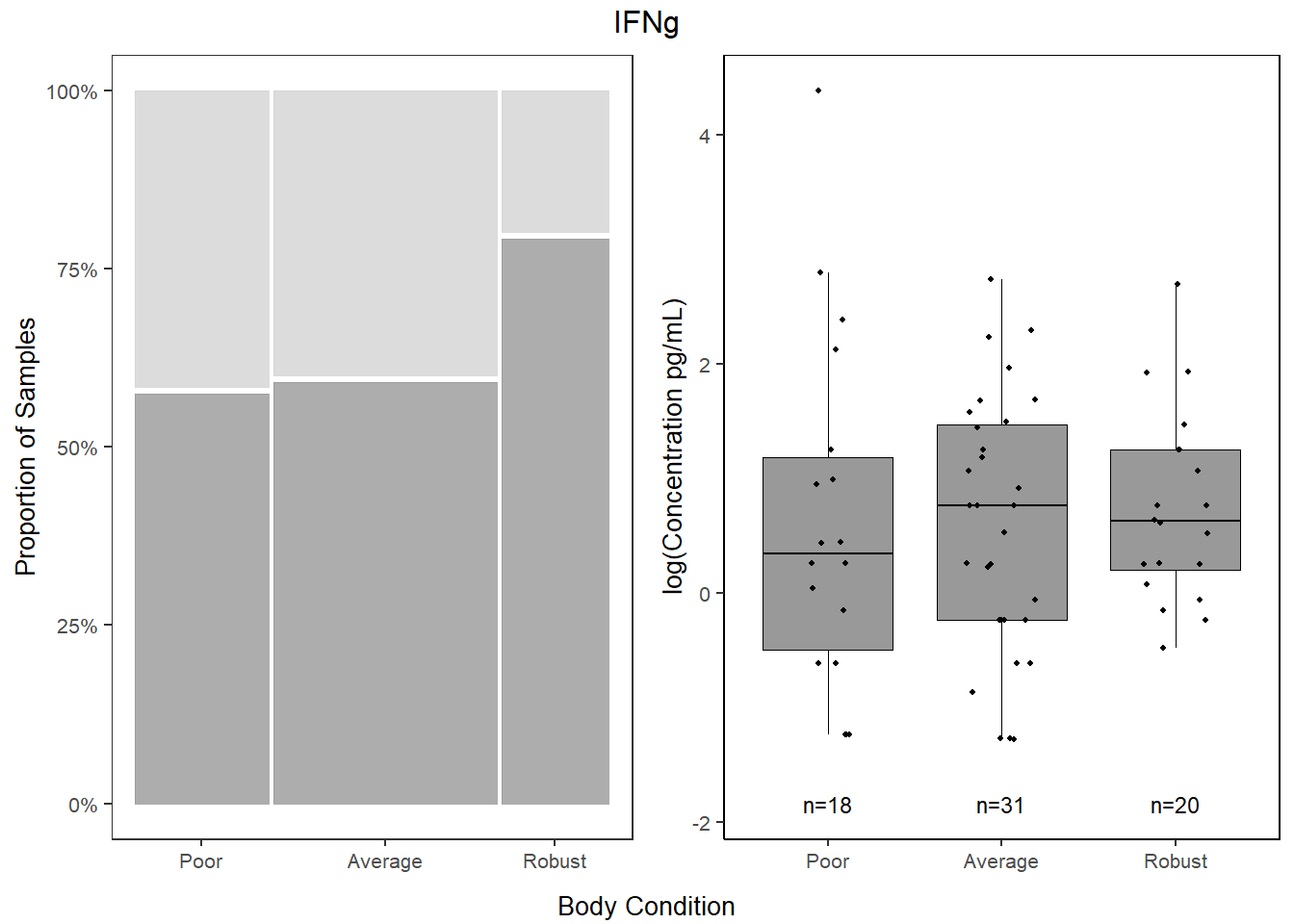

bottom <- grid.arrange(cyto, cyto_leg, 
                       ncol=1, 
                       heights=c(3,0.5))

jpeg("Figures/cytoimportance_bodycondition.jpeg", width=7, height=6, units="in", res=300)
all <- grid.arrange(varimp_plot, bottom, 
                    heights=c(1.25,2))
grid.polygon(x=c(0, 0, 1, 1),
             y=c(0, 0.62, 0.62, 0),
             gp=gpar(fill=NA))
grid.polygon(x=c(0.02, 0.02, 0.97, 0.97),
             y=c(0.955, 0.99, 0.99, 0.955),
             gp=gpar(fill=NA))
dev.off()

## png 
##   2