6 IAV ~ cytokines

6.1 Libraries

library(vegan)
library(mixOmics)
library(tidyverse)
library(pairwiseAdonis)
library(mlr3)
library(mlr3tuning)
library(rpart)
library(rpart.plot)
library(ggmosaic)
library(ggpubr)
library(EnvStats)
library(gridExtra)
library(grid)
library(PLSDAbatch)

6.2 Data

cyto <- 
  read.csv("Output Files/cleaned_cytokine.csv")
cytobin <- 
  read.csv("Output Files/cleaned_cytokine_bin.csv")

meta <- read.csv("Output Files/metadata_cyto.csv") %>% 
  mutate(iav=gsub("neg", "IAV-", iav),
         iav=gsub("pos", "IAV+", iav))

# Merge cytokine & metadata 
data <- merge(cyto, meta, by="Sample") %>% 
  filter(!is.na(iav)) %>% 
  mutate(analysis.year=factor(analysis.year))

databin <- 
  merge(cytobin, meta, by="Sample") %>% 
  filter(!is.na(iav)) %>% 
  mutate(analysis.year=factor(analysis.year))

6.3 PERMANOVA

6.3.1 Cytokine Presence/Absence

6.3.1.1 Create similarity matrix (Sorensen)

Dissimilarity = 1-Sorensen

databin_dist <- 
  databin %>% 
  select(2:10) %>% 
  betadiver(., method=11)

plot((1-databin_dist))

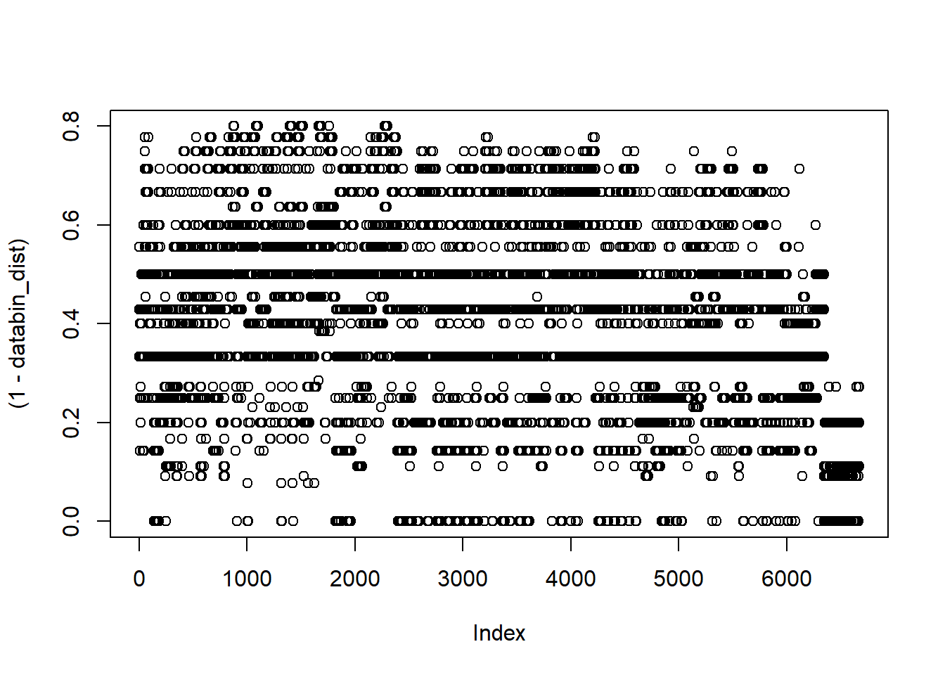
# Dissimilarity summary stats
mean(1-databin_dist); min(1-databin_dist); max(1-databin_dist); median(1-databin_dist)

## [1] 0.4016769

## [1] 0

## [1] 0.8

## [1] 0.4

6.3.1.2 Run PERMANOVA

Use restricted permutation test - data are not exchangeable between analysis years so permute within groups defined by strata.
** Not sig

# define permutations & strata
permute_databin <- 
  how(plots=Plots(strata=databin$analysis.year, type="none"), nperm=4999)

# run permanova
adonis2((1-databin_dist) ~ iav, 
        data=databin,
        permutations=permute_databin)

## Permutation test for adonis under reduced model
## Plots: databin$analysis.year, plot permutation: none
## Permutation: free
## Number of permutations: 4999
## 
## adonis2(formula = (1 - databin_dist) ~ iav, data = databin, permutations = permute_databin)
##           Df SumOfSqs      R2      F Pr(>F)
## Model      1   0.3814 0.03362 3.9657 0.1828
## Residual 114  10.9638 0.96638              
## Total    115  11.3452 1.00000

6.3.1.3 Homogeneity of group dispersions

** Not sig

disper <- 
  betadisper((1-databin_dist), group=databin$iav, type="centroid")

anova(disper)

## Analysis of Variance Table
## 
## Response: Distances
##            Df  Sum Sq   Mean Sq F value Pr(>F)
## Groups      1 0.00374 0.0037435  0.4087 0.5239
## Residuals 114 1.04431 0.0091606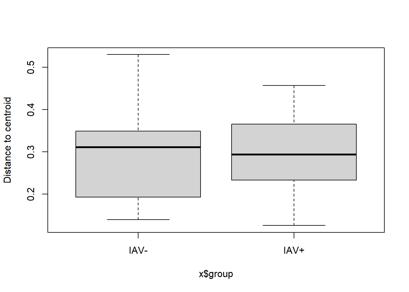

boxplot(disper)

6.3.1.4 Visualization

Principal Coordinates Analysis

# Use 1 - Sorensen's for dissimilarity 
databin_pco <- cmdscale(1-databin_dist, eig=TRUE)

plot(databin_pco$points, type="n", 
     cex.lab=1.5, cex.axis=1.1, cex.sub=1.1)
ordiellipse(ord = databin_pco, 
            groups = factor(data$iav), 
            display = "sites", 
            col = c("grey", "darkseagreen"),
            lwd = 2,
            label = TRUE)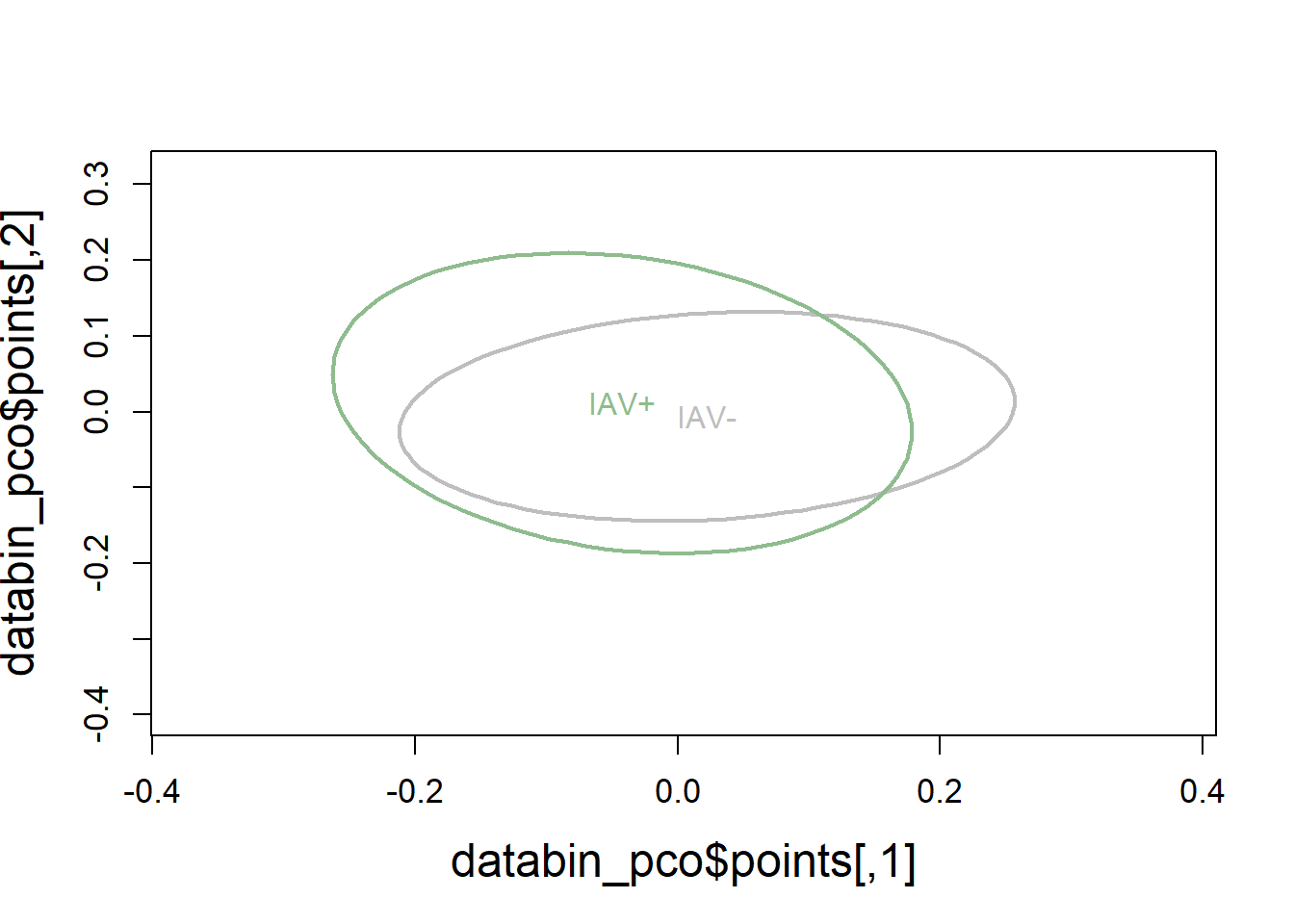

plot(databin_pco$points, type="n", 
     cex.lab=1.5, cex.axis=1.1, cex.sub=1.1)
ordispider(ord = databin_pco,
           groups = factor(data$iav),
           display = "sites",
           col = c("grey", "darkseagreen"),
           lwd=2,
           label=TRUE)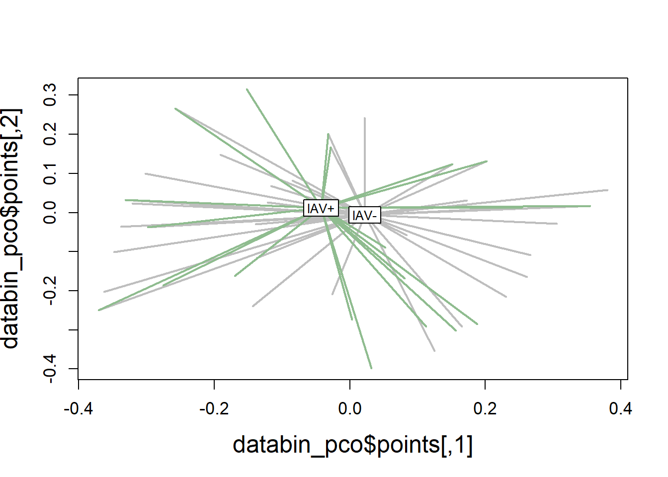

6.3.2 Cytokine Concentration

6.3.2.1 Dissimilarity matrix

data_dist <-
  data %>% 
  select(2:10) %>% 
  vegdist(., method="bray")

6.3.2.2 Run PERMANOVA

** Not sig

# define permutations & strata
permute_data <- 
  how(plots=Plots(strata=data$analysis.year, type="none"),
      nperm=4999)

# run permanova
adonis2(data_dist ~ iav, 
        data=data,
        permutations=permute_data)

## Permutation test for adonis under reduced model
## Plots: data$analysis.year, plot permutation: none
## Permutation: free
## Number of permutations: 4999
## 
## adonis2(formula = data_dist ~ iav, data = data, permutations = permute_data)
##           Df SumOfSqs      R2      F Pr(>F)
## Model      1   0.2609 0.01366 1.5784  0.477
## Residual 114  18.8403 0.98634              
## Total    115  19.1011 1.00000

6.3.2.3 Homogeneity of group dispersions

** Not sig

disper <- 
  betadisper(data_dist, group=data$iav, type="centroid")

anova(disper)

## Analysis of Variance Table
## 
## Response: Distances
##            Df  Sum Sq  Mean Sq F value Pr(>F)  
## Groups      1 0.09537 0.095372  3.6232 0.0595 .
## Residuals 114 3.00074 0.026322                 
## ---
## Signif. codes:  0 '***' 0.001 '**' 0.01 '*' 0.05 '.' 0.1 ' ' 1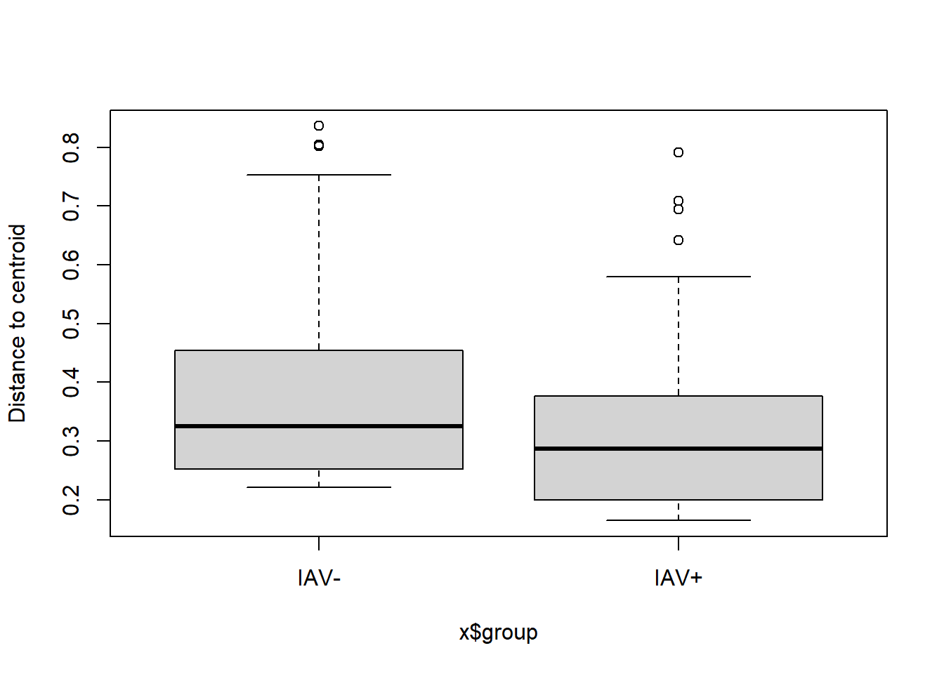

boxplot(disper)

6.3.2.4 Visualization

# Use Bray-Curtis dissimilarity matrix
data_pco <- cmdscale(data_dist, eig=TRUE)

plot(data_pco$points, type="n", 
     cex.lab=1.5, cex.axis=1.1, cex.sub=1.1)
ordiellipse(ord = data_pco, 
            groups = factor(data$iav), 
            display = "sites", 
            col = c("grey", "darkseagreen"),
            lwd = 2,
            label = TRUE)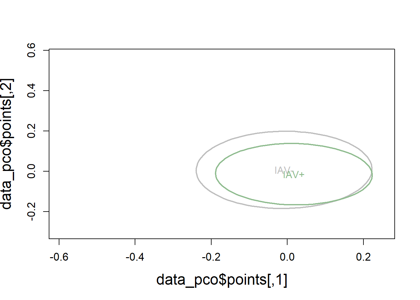

plot(data_pco$points, type="n", 
     cex.lab=1.5, cex.axis=1.1, cex.sub=1.1)
ordispider(ord = data_pco,
           groups = factor(data$iav),
           display = "sites",
           col = c("grey", "darkseagreen"),
           lwd=2,
           label=TRUE)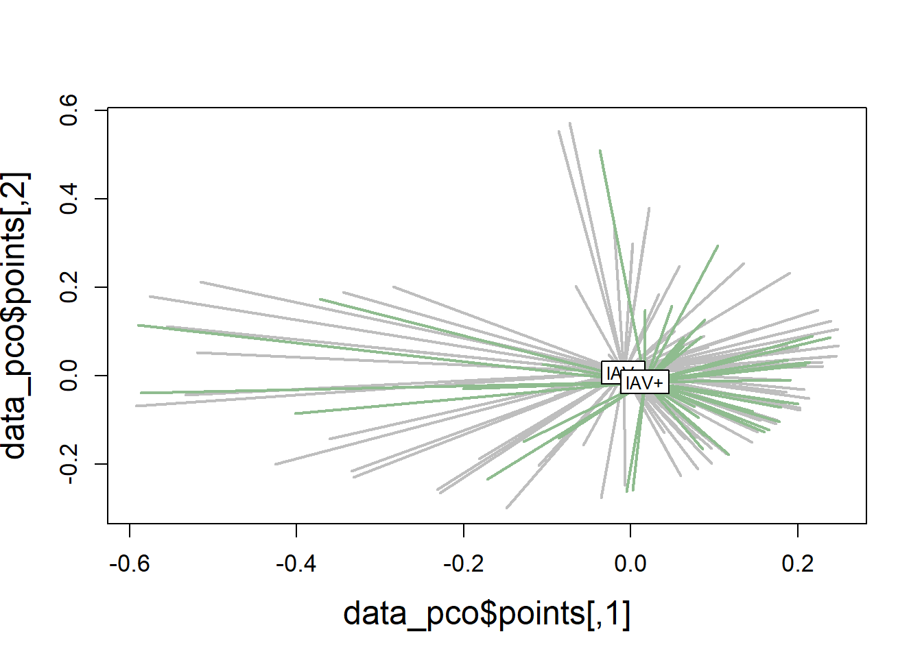

6.4 PLS-DA

6.4.1 Data

pls_x <-
 data[,1:10] %>% 
  column_to_rownames(var = "Sample")

pls_y <- 
  data %>% 
  mutate(iav=gsub("neg", "IAV-", iav),
         iav=gsub("pos", "IAV+", iav),
         iav=as.factor(iav)) %>% 
  select(Sample, iav, analysis.year)  %>% 
  column_to_rownames(var = "Sample")

6.4.2 Transform data

CLR = Centered log-ratio transformation

pls_x_clr <- 
  logratio.transfo(X = pls_x, logratio = 'CLR', offset = 0.01)

class(pls_x_clr) = 'matrix'

6.4.3 Detect batch effect

Reference: https://evayiwenwang.github.io/PLSDAbatch_workflow/

pca_before <- 
  mixOmics::pca(pls_x_clr, scale=TRUE)

plotIndiv(pca_before, 
          group=data$analysis.year,
          pch=20,
          legend = TRUE, legend.title = "Analysis Year",
          title = "Before Batch Correction",
          ellipse = TRUE, ellipse.level=0.95)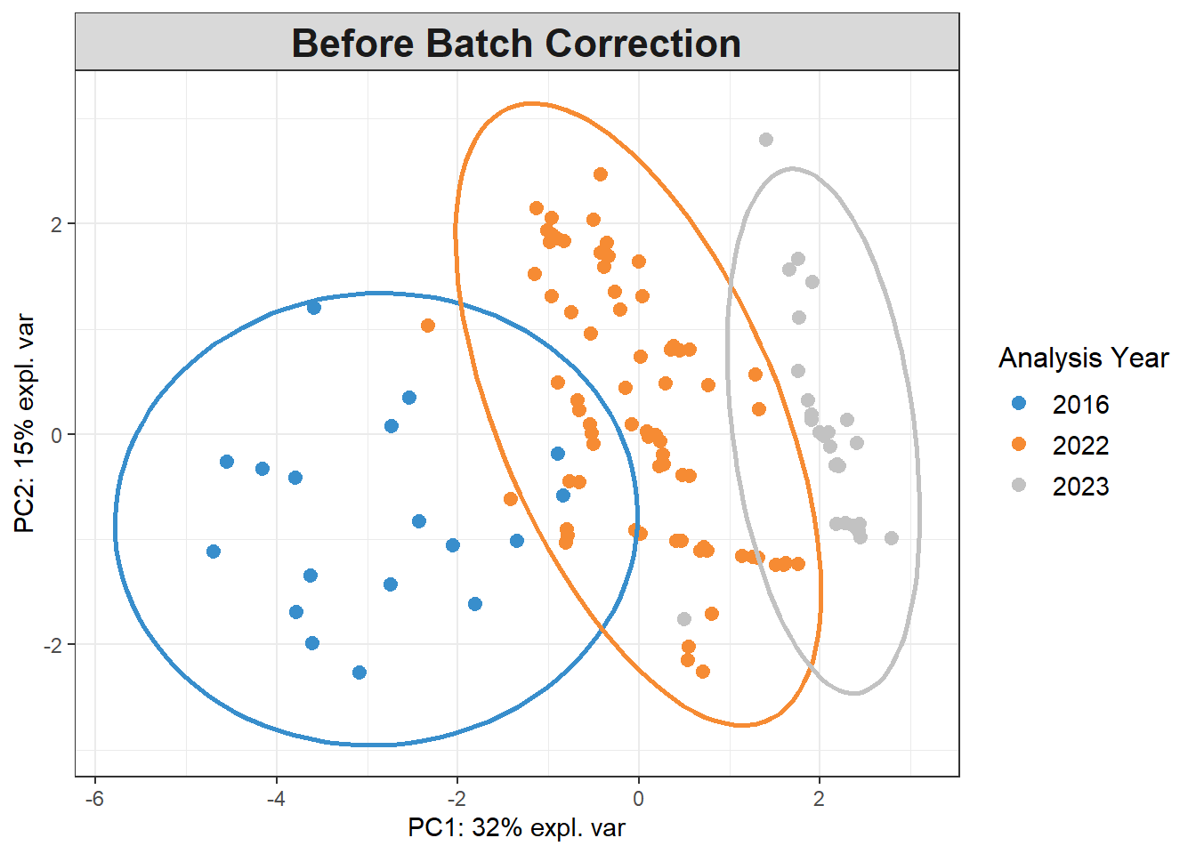

Scatter_Density(object = pca_before,
                batch = pls_y$analysis.year,
                trt = pls_y$bc_bin,
                trt.legend.title = "Body Condition",
                color.set = c("#9d9d9d","#008ba2","black"))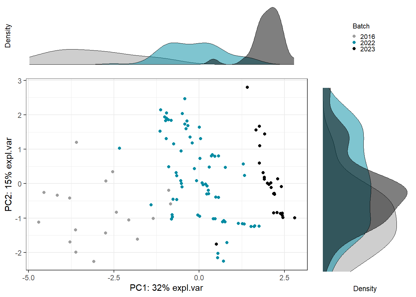

6.4.3.1 Estimate # variable components

Use PLSDA from mixOmics with only treatment to choose number of treatment components to preserve.
Number = that explains 100% of variance in outcome matrix Y.

trt_comp <- 
  plsda(X = pls_x_clr,
        Y = pls_y$iav, 
        ncomp=9)

trt_comp$prop_expl_var

## $X
##      comp1      comp2      comp3      comp4      comp5      comp6      comp7 
## 0.17471622 0.25676902 0.11055489 0.09763907 0.07510012 0.06899208 0.12441304 
##      comp8      comp9 
## 0.09181557 0.08605453 
## 
## $Y
##     comp1     comp2     comp3     comp4     comp5     comp6     comp7     comp8 
## 1.0000000 0.8351838 0.8094240 0.8042025 0.8033727 0.8029372 0.8029271 0.8029271 
##     comp9 
## 0.8029271

sum(trt_comp$prop_expl_var$Y[seq_len(1)]) # preserve 1 comp

## [1] 1

6.4.3.2 Estimate # batch components

Use PLSDA_batch with both treatment and batch to estimate optimal number of batch components to remove.
For ncomp.trt, use # components found above. Samples are not balanced across batches x treatment, using balance = FALSE.
Choose # that explains 100% variance in outcome matrix Y.

batch_comp <- 
  PLSDA_batch(X = pls_x_clr,
              Y = pls_y$iav,
              Y.bat = pls_y$analysis.year,
              balance = FALSE,
              ncomp.trt = 1, ncomp.bat = 9)

batch_comp$explained_variance.bat

## $X
##      comp1      comp2      comp3      comp4      comp5      comp6      comp7 
## 0.50875836 0.11640179 0.07128088 0.14655103 0.05411045 0.07033902 0.03255846 
##      comp8      comp9 
## 0.11079636 0.01760352 
## 
## $Y
##      comp1      comp2      comp3      comp4      comp5      comp6      comp7 
## 0.39147326 0.55682867 0.05169808 0.39135410 0.55354977 0.05376613 0.54820462 
##      comp8      comp9 
## 0.39556449 0.05306025

sum(batch_comp$explained_variance.bat$Y[seq_len(3)]) # preserve 3 comp

## [1] 1

6.4.3.3 Correct for batch effects

Use optimal number of components determined above.
Treatment = 1, Batch = 3

plsda_batch <-
  PLSDA_batch(X = pls_x_clr,
              Y = pls_y$iav,
              Y.bat = pls_y$analysis.year,
              balance = FALSE,
              ncomp.trt = 1, ncomp.bat = 3)

data_batch_matrix <-
  plsda_batch$X.nobatch

data_batch_df <- 
  data_batch_matrix %>% 
  data.frame() %>% 
  mutate(iav = pls_y$iav)

write.csv(data_batch_df, "Output Files/batchcorrected_iav.csv")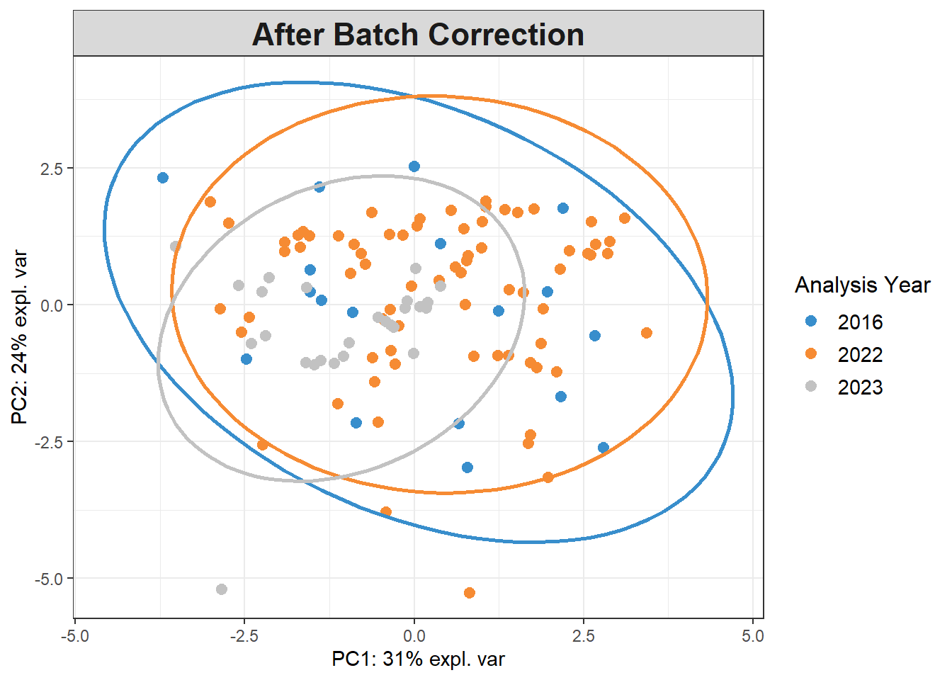

6.4.3.4 Assessing batch correction

after_batch <- 
  mixOmics::pca(data_batch_matrix, scale=TRUE)

plotIndiv(after_batch, 
          group=pls_y$analysis.year,
          pch=20, 
          legend = TRUE, legend.title = "Analysis Year",
          title = "After Batch Correction",
          ellipse = TRUE, ellipse.level = 0.95)

6.4.4 PLSDA on Batch-Corrected Data

plsda_model <- 
  plsda(data_batch_matrix,
        pls_y$iav,
        scale=TRUE)

plotIndiv(plsda_model,
          group=pls_y$iav,
          pch=20, 
          legend = TRUE, legend.title = "IAV Status",
          ellipse = TRUE, ellipse.level = 0.95)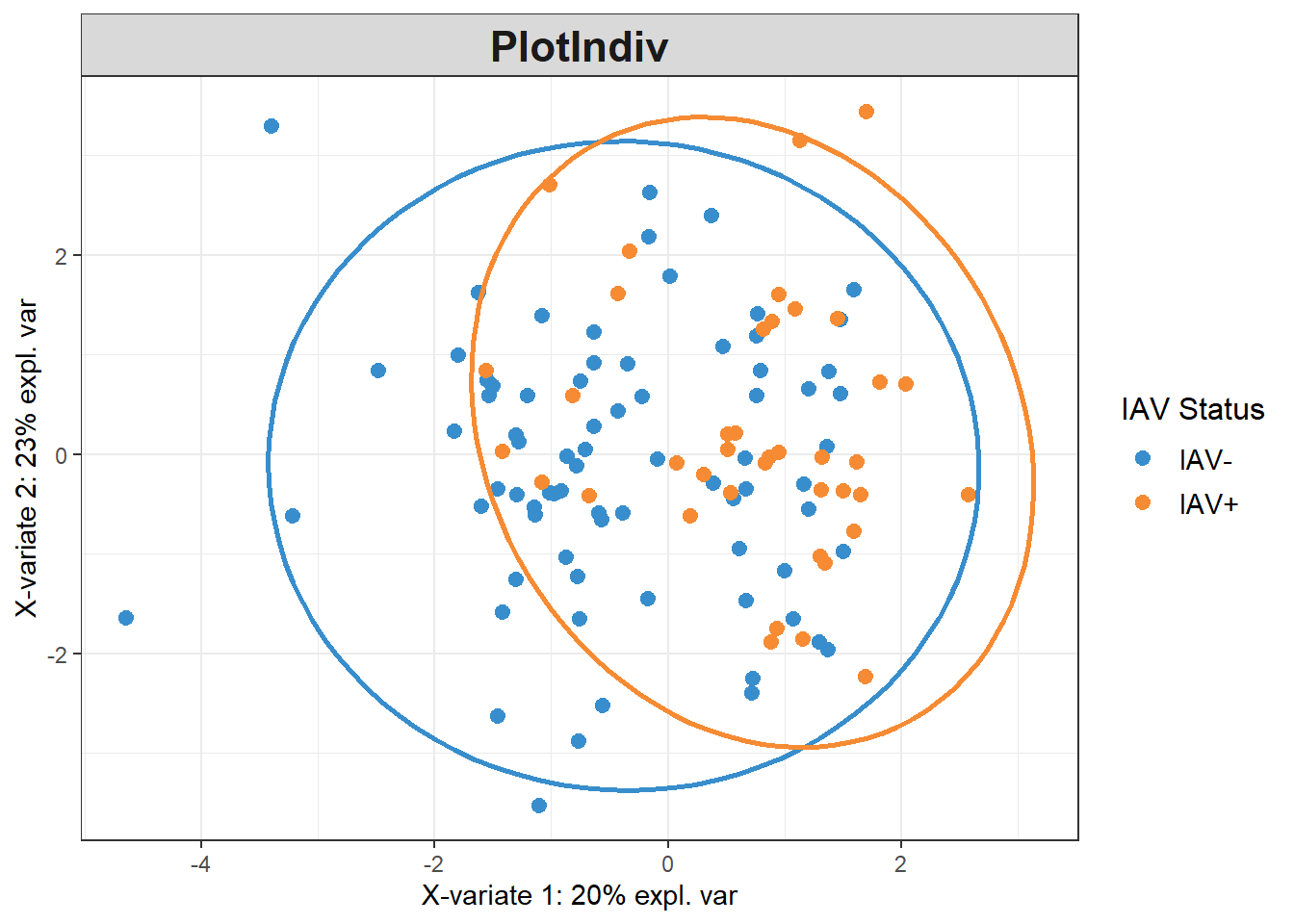

6.4.5 Visualizations

6.4.5.1 Set x and y axis labels

labelx <- 
  paste("X-variate 1: ", 
        round(abs(plsda_model$prop_expl_var$X[1]*100), digits=0),
        "% expl. var",
        sep="")

labely <- 
  paste("X-variate 2: ", 
        round(abs(plsda_model$prop_expl_var$X[2]*100), digits=0),
        "% expl. var",
        sep="")

6.4.5.2 Create plot data frame

plsda_ggplot <- 
  data.frame(x = plsda_model$variates$X[,1], 
             y = plsda_model$variates$X[,2],
             iav = plsda_model$Y,
             analysis.year=factor(pls_y$analysis.year))

6.4.5.3 Plot

iav_plsda_ggplot <- 
  ggplot(plsda_ggplot, 
         aes(x=x, 
             y=y,
             col=iav)) +
  geom_point() +
  stat_ellipse() +
  labs(x=labelx,
       y = labely,
       name="IAV Status") +
  scale_color_manual("IAV Status",
                     values=c("#9d9d9d","#008ba2")) +
  theme_bw() +
  theme(panel.grid=element_blank())

iav_plsda_ggplot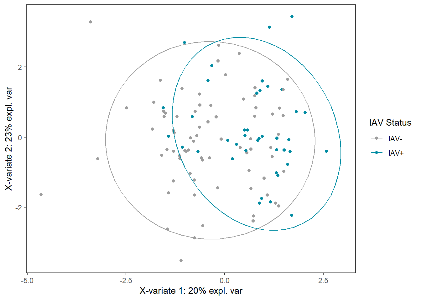

6.4.5.4 Presentation Plot

# Presentation
iav_plsda_pres <- 
   ggplot(plsda_ggplot, 
         aes(x=x, 
             y=y,
             col=iav)) +
  geom_point() +
  stat_ellipse() +
  labs(x=labelx,
       y = labely,
       name="IAV Status") +
  scale_color_manual("IAV Status",
                     values=c("#9d9d9d","#7FC1DB")) +
  theme_bw() +
  theme(panel.grid=element_blank(),
        legend.position = "bottom", 
        text = element_text(size = 18))
iav_plsda_pres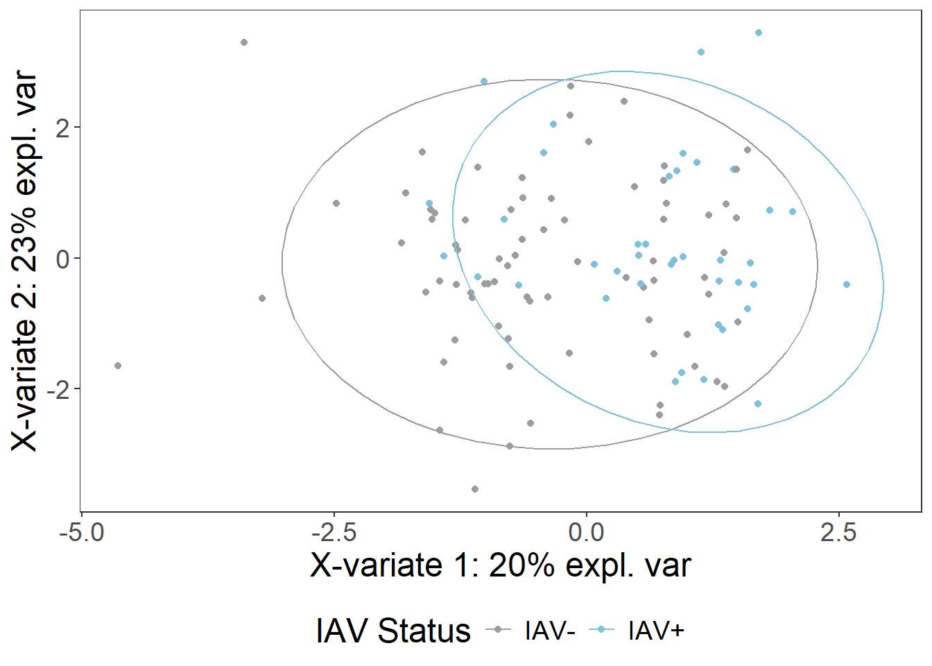

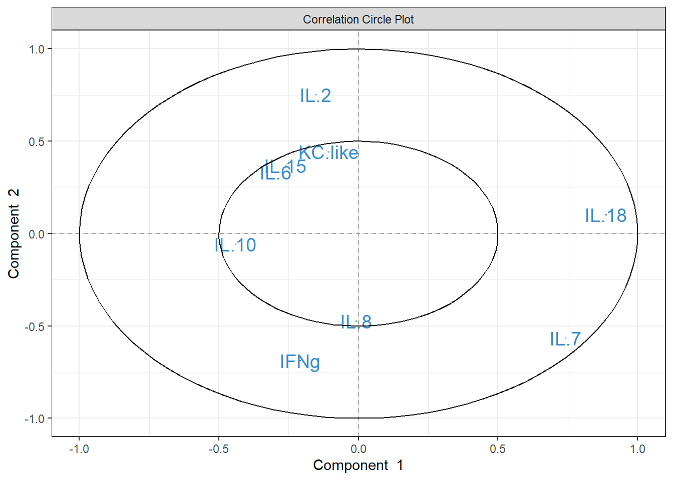
ggsave("Figures/IAV_presentation.jpeg", iav_plsda_pres,
       width = 6, height = 5, units = "in")

6.4.6 Cytokine Contributions

plsda_loadings <- 
  plsda_model$loadings$X %>% 
  data.frame() %>% 
  select(1:2) %>% 
  arrange(comp1)
plsda_loadings

##                comp1       comp2
## IL.10   -0.339760020  0.02332628
## IFNg    -0.295663429 -0.43075479
## IL.8    -0.165618911 -0.52182239
## IL.6    -0.135013840  0.32427925
## IL.15   -0.073708934  0.43507606
## KC.like -0.009718823  0.24376693
## IL.2    -0.007987815  0.36859902
## IL.7     0.513862191 -0.22747648
## IL.18    0.694148605 -0.01123763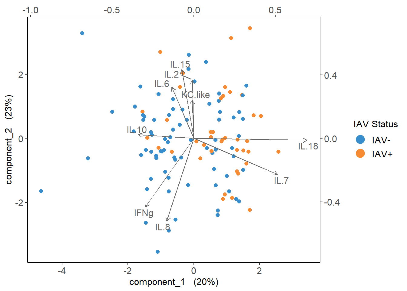

biplot(plsda_model, ind.names=FALSE, legend.title="IAV Status")

plotVar(plsda_model)

6.5 CART

Cytokine Importance ### Prepare data

data_cart <- 
  data %>% 
  select(2:10, iav) %>% 
  mutate(iav=factor(iav))

6.5.1 Cross Validation

# Creating task and learner
task <- as_task_classif(iav ~ ., 
                        data = data_cart)
        
task <- task$set_col_roles(cols="iav",
                           add_to="stratum")

learner <- lrn("classif.rpart",
               predict_type = "prob",
               maxdepth = to_tune(2, 5),
               minbucket = to_tune(1, 40),
               minsplit = to_tune(1, 30)
               )

# Define tuning instance - info ~ tuning process
instance <- ti(task = task,
               learner = learner,
               resampling = rsmp("cv", folds = 10),
               measures = msr("classif.ce"),
               terminator = trm("none")
               )

# Define how to tune the model
tuner <- tnr("grid_search", 
             batch_size = 10
             )

# Trigger the tuning process
#tuner$optimize(instance)

# optimal values: 
  # maxdepth = 5
  # minbucket = 9
  # minsplit = 20
  # classif.ce = 0.2909091

6.5.2 Run model with optimized parameters

cart_model <- rpart(formula=iav ~ .,
                    data=data_cart,
                    method="class",
                    maxdepth=5,
                    minbucket=9,
                    minsplit=20)

# plot optimized tree
rpart.plot(cart_model)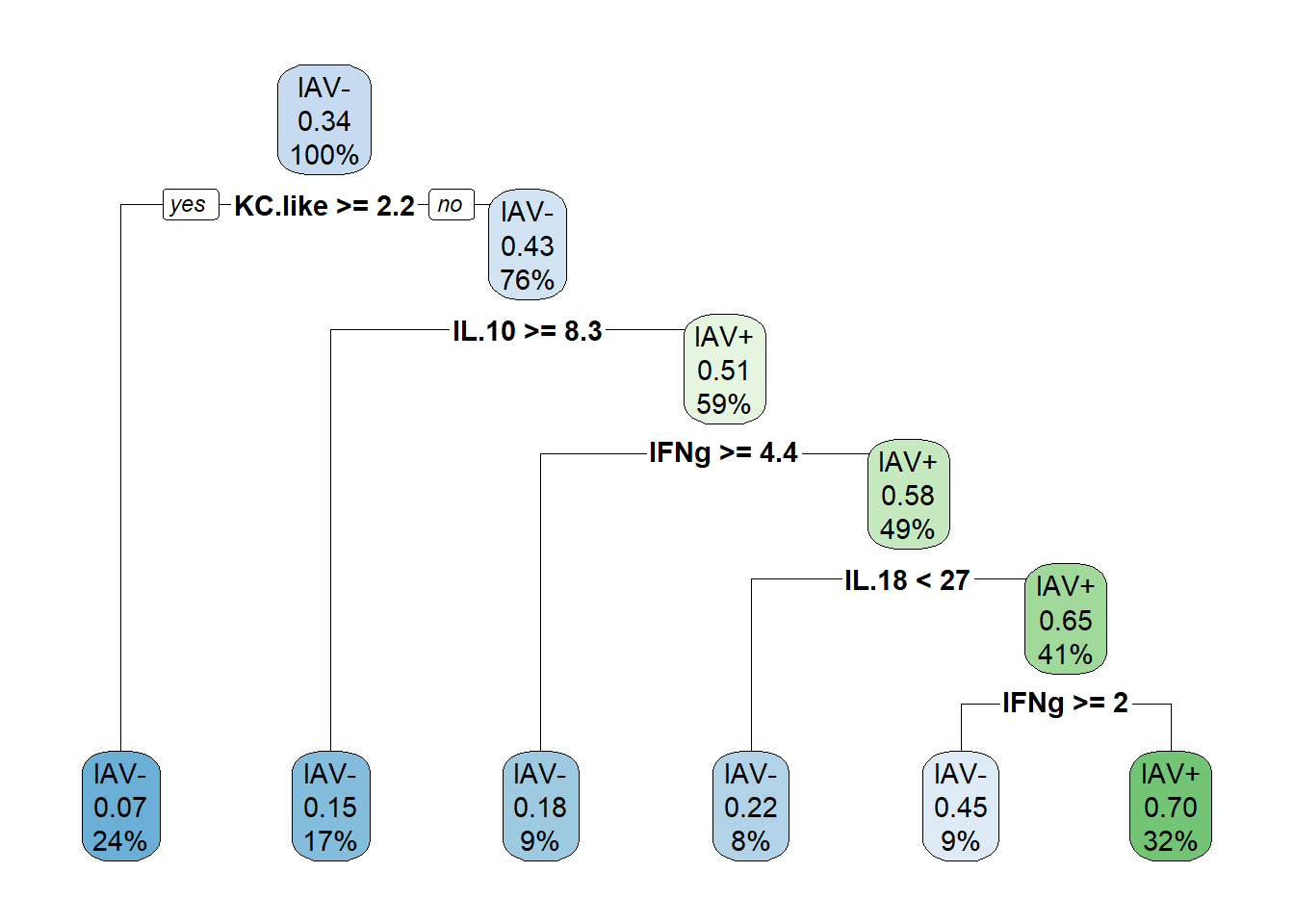

cart_model$variable.importance 

##    KC.like       IL.6      IL.18       IFNg      IL.10       IL.8      IL.15 
## 5.78208805 4.53238756 4.15895972 4.15827720 4.11122995 1.43893048 0.41112299 
##       IL.2 
## 0.09493895

  # KC-like, IL-6 are top two cytokines

6.5.3 Plot

Variable importance: the sum of the goodness of split measures for each split for which it was the primary variable, plus goodness * (adjusted agreement) for all splits in which it was a surrogate. In the printout these are scaled to sum to 100 and the rounded values are shown, omitting any variable whose proportion is less than 1%. (https://cran.r-project.org/web/packages/rpart/vignettes/longintro.pdf)

6.5.3.1 Variable Importance

varimp <- 
  data.frame(imp=cart_model$variable.importance) %>% 
  rownames_to_column() %>% 
  rename("variable" = rowname) %>% 
  arrange(imp) %>%
  mutate(variable=gsub("\\.","-",variable),
         variable = forcats::fct_inorder(variable))

varimp_plot <- 
  ggplot(varimp) + 
  geom_segment(aes(x = variable, 
                   y = 0, 
                   xend = variable, 
                   yend = imp), 
               linewidth = 0.5, 
               alpha = 0.7) +
  geom_point(aes(x = variable, 
                 y = imp), 
             size = 1, 
             show.legend = F,
             col="black") +
  labs(x="Cytokine", 
       y="Variable Importance") +
  coord_flip() +
  theme_classic() +
  theme(text=element_text(size=10, color="black"))

6.5.3.2 Data Prep

databin <-
  databin %>% 
  mutate(across(2:10, \(x) gsub("1", "Present", x)),
         across(2:10, \(x) gsub("0", "Absent", x)),
         across(2:10, \(x) factor(x, levels=c("Present", "Absent"))))

6.5.3.3 Proportions

prop.table(table(databin$iav, databin$KC.like), margin=1)*100

##       
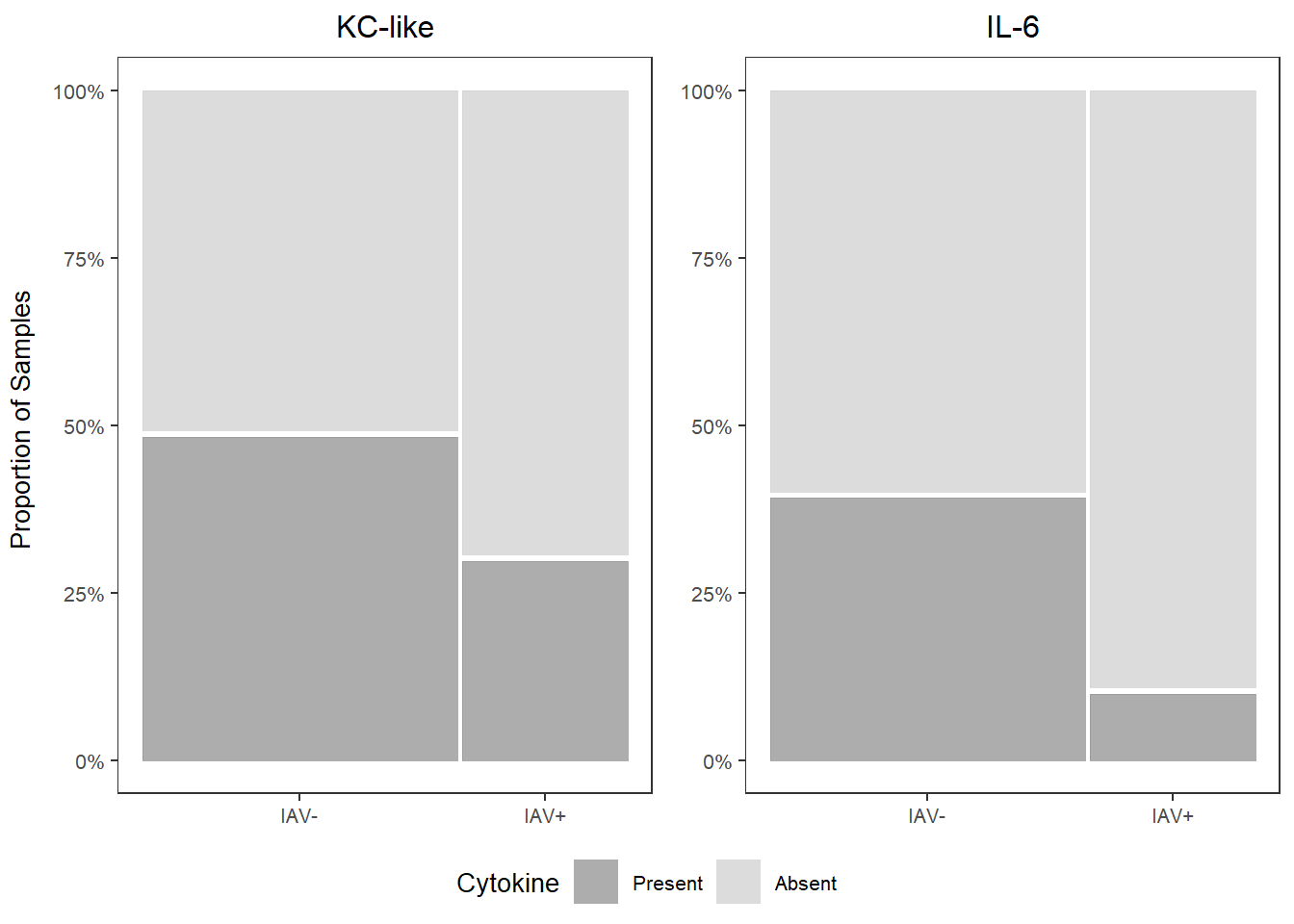
##         Present   Absent
##   IAV- 48.68421 51.31579
##   IAV+ 30.00000 70.00000

prop.table(table(databin$iav, databin$IL.6), margin=1)*100

##       
##         Present   Absent
##   IAV- 39.47368 60.52632
##   IAV+ 10.00000 90.00000

kc_prop <- 
  databin %>%
  ggplot(data=.) +
  geom_mosaic(aes(x=product(KC.like,iav), fill=KC.like)) +
  scale_fill_manual(values=c("Present"="gray60", "Absent"="lightgray"),
                    name="Cytokine") +
  scale_y_continuous(labels = scales::percent) +
  labs(title="KC-like") +
  theme_bw() +
  theme(panel.grid.major = element_blank(), 
        panel.grid.minor = element_blank(),
        axis.title.x = element_blank(),
        axis.title.y = element_blank(),
        legend.position="bottom",
        text = element_text(size=10),
        plot.title = element_text(hjust = 0.5))
kc_prop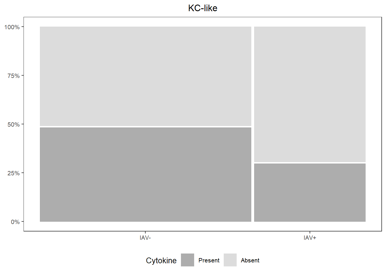

cyto_leg <- get_legend(kc_prop)

kc_prop <-
  kc_prop +
  theme(legend.position="none")

il6_prop <- 
  databin %>%
  ggplot(data=.) +
  geom_mosaic(aes(x=product(IL.6,iav), fill=IL.6)) +
  scale_fill_manual(values=c("Present"="gray60", "Absent"="lightgray")) +
  scale_y_continuous(labels = scales::percent) +
  labs(title="IL-6") +
  theme_bw() +
  theme(panel.grid.major = element_blank(), 
        panel.grid.minor = element_blank(),
        axis.title.x = element_blank(), 
        axis.title.y = element_blank(),
        legend.position="none",
        text = element_text(size=10),
        plot.title = element_text(hjust = 0.5))
il6_prop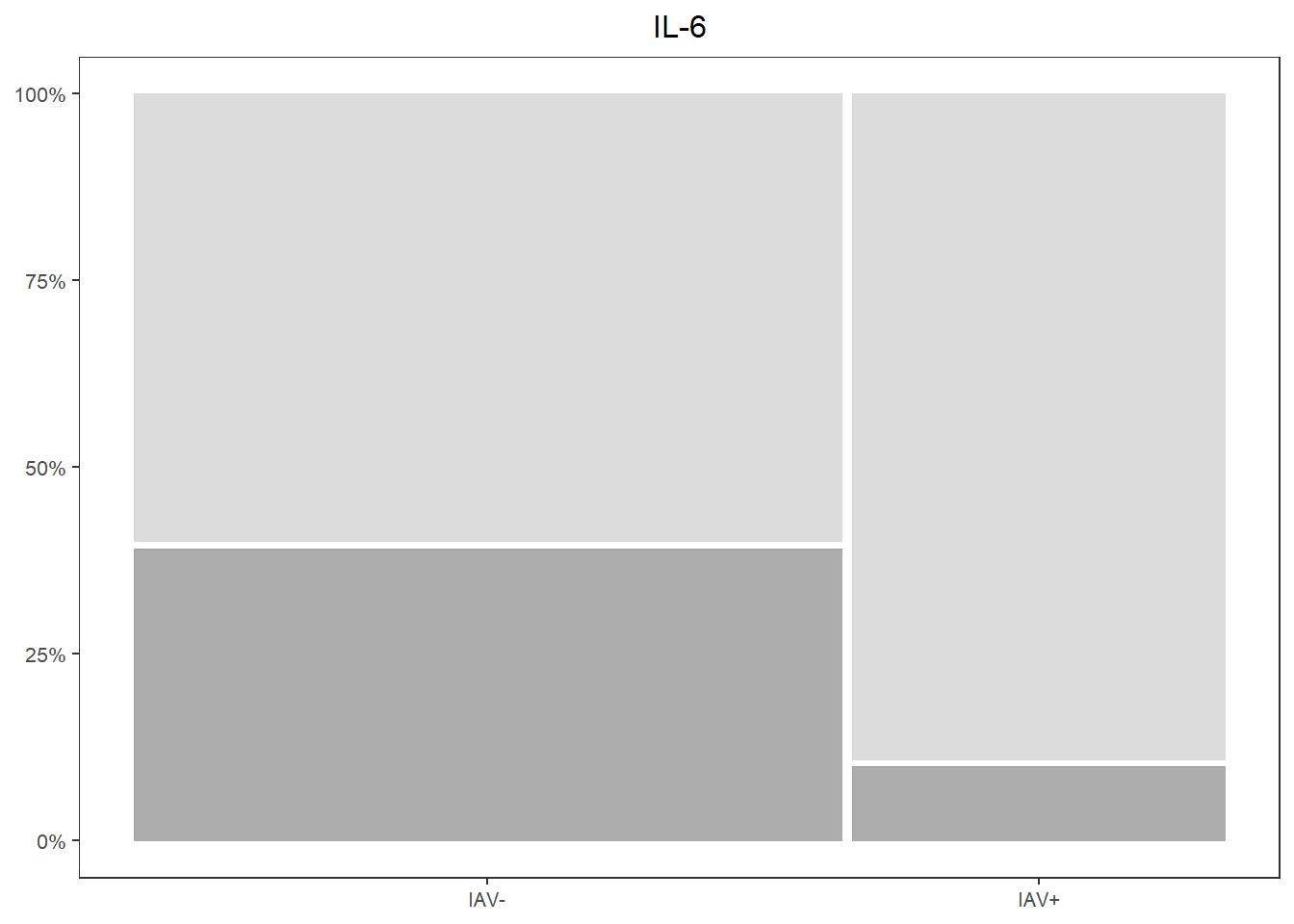

6.5.3.4 Concentrations

kclike <- 
  data %>% 
  select(iav, KC.like) %>% 
  filter(!KC.like==0) %>% 
  ggplot(., aes(x=iav, y=log(KC.like))) +
  geom_boxplot(color="black", fill="gray60", lwd=0.25,
               outliers=FALSE) +
  geom_point(size=0.75, position=position_jitter(width=0.2)) +
  labs(x=NULL, y=NULL) +
  stat_n_text(size=3) +
  theme_classic() +
  theme(text = element_text(size=10),
         panel.border=element_rect(color="black", fill=NA, linewidth=0.5))
kclike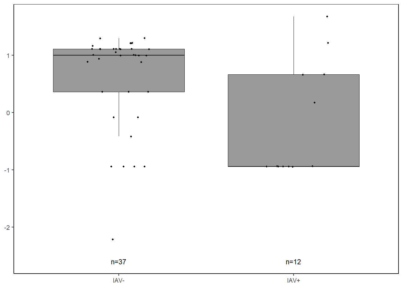

il6 <- 
  data %>% 
  select(iav, IL.6) %>% 
  filter(!IL.6 == 0) %>% 
  ggplot(., aes(x=iav, y=log(IL.6))) +
  geom_boxplot(color="black", fill="gray60", lwd=0.25,
               outliers=FALSE) +
  geom_point(size=0.75, position=position_jitter(width=0.2)) +
  labs(x=NULL, y=NULL) +
  stat_n_text(size=3) +
  theme_classic() +
  theme(text = element_text(size=10),
        panel.border=element_rect(color="black", fill=NA, linewidth=0.5))
il6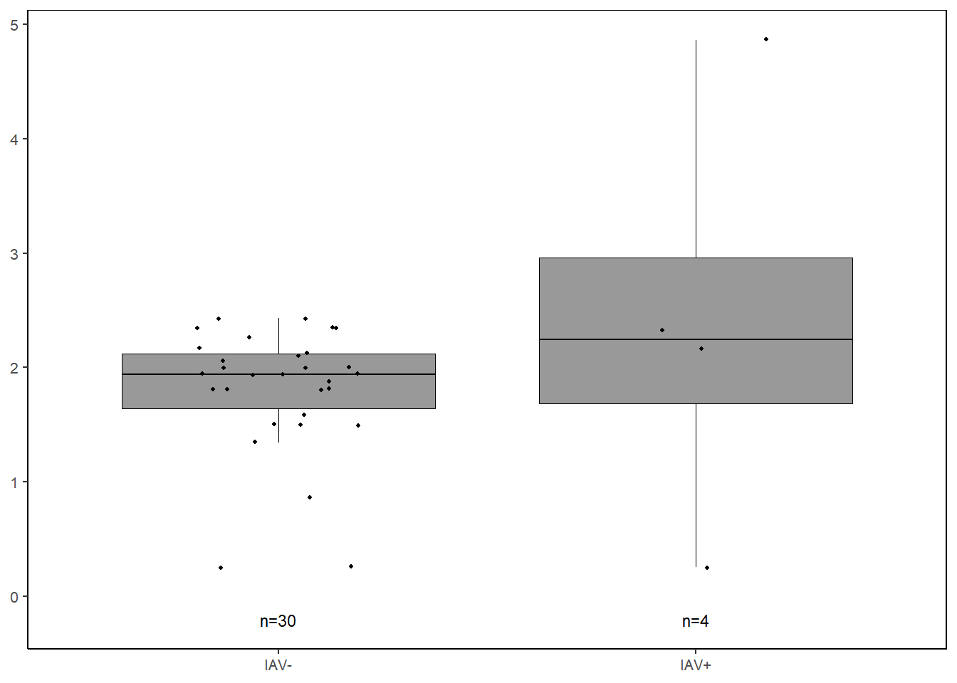

6.5.3.5 Combine together

prop_grid <- grid.arrange(kc_prop, il6_prop, ncol=2,
                          left=textGrob("Proportion of Samples",
                                        rot=90, gp=gpar(fontsize=10)))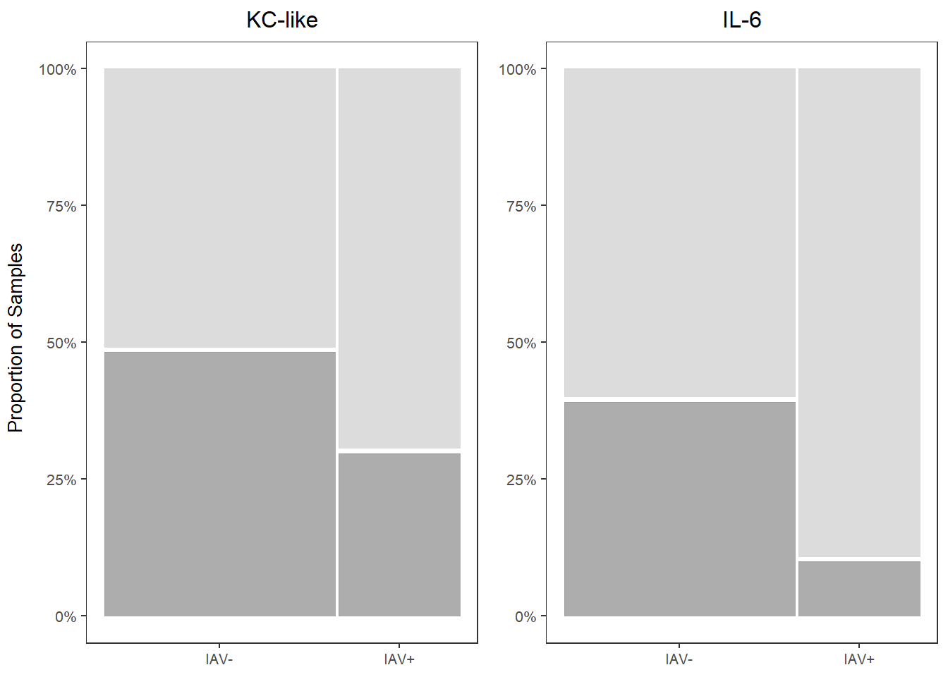

prop_grid2 <- grid.arrange(prop_grid, cyto_leg,
                          ncol=1, 
                          heights=c(3, 0.3))

conc_grid <- grid.arrange(kclike, il6, ncol=2, 
                          left=textGrob("log(Concentration (pg/mL))", 
                                        rot=90, gp=gpar(fontsize=10)))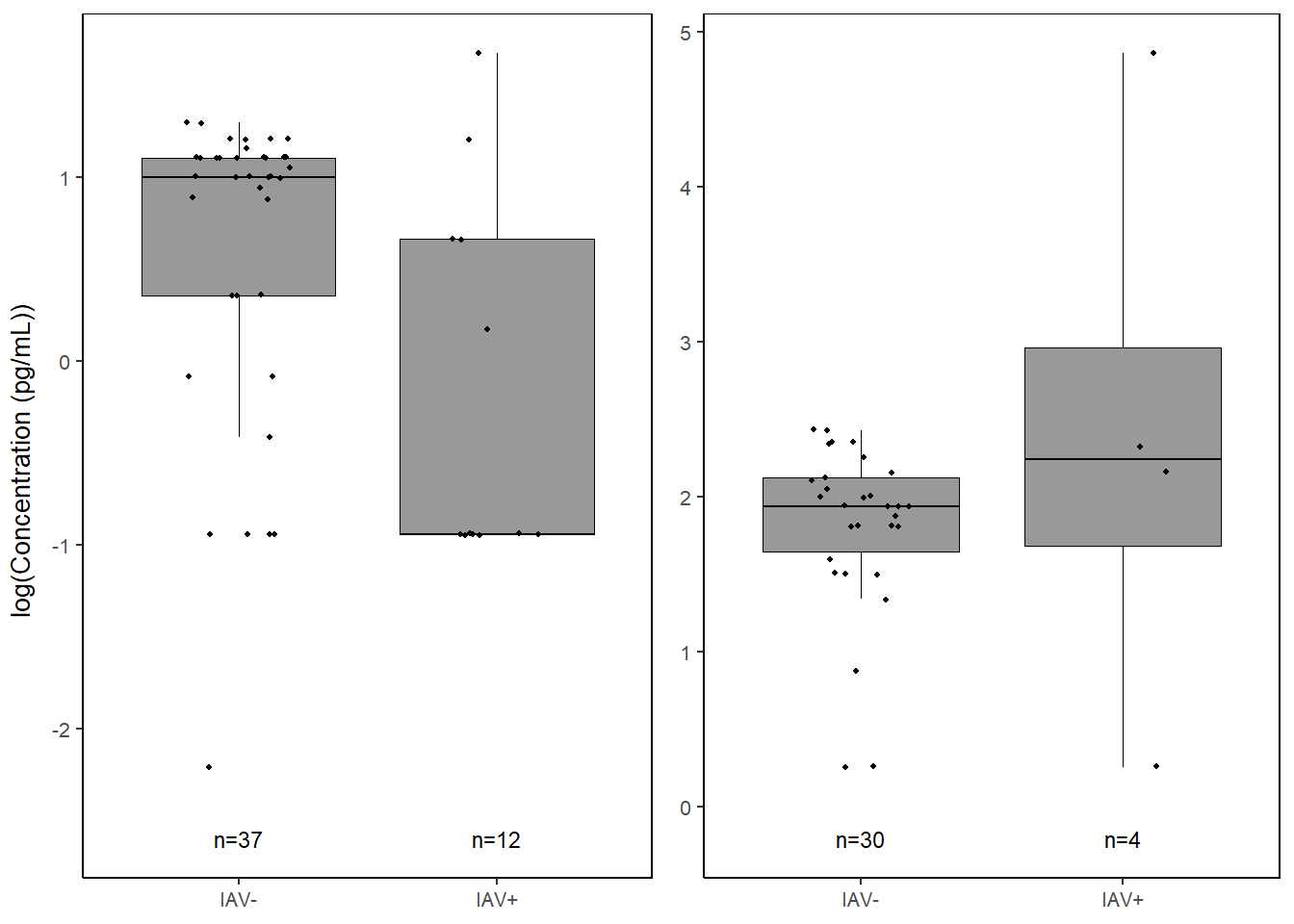

cyto_grid <- grid.arrange(prop_grid2, conc_grid,
                          ncol=1, 
                          heights=c(4,3.5),
                          bottom=textGrob("IAV Status", gp=gpar(fontsize=10)))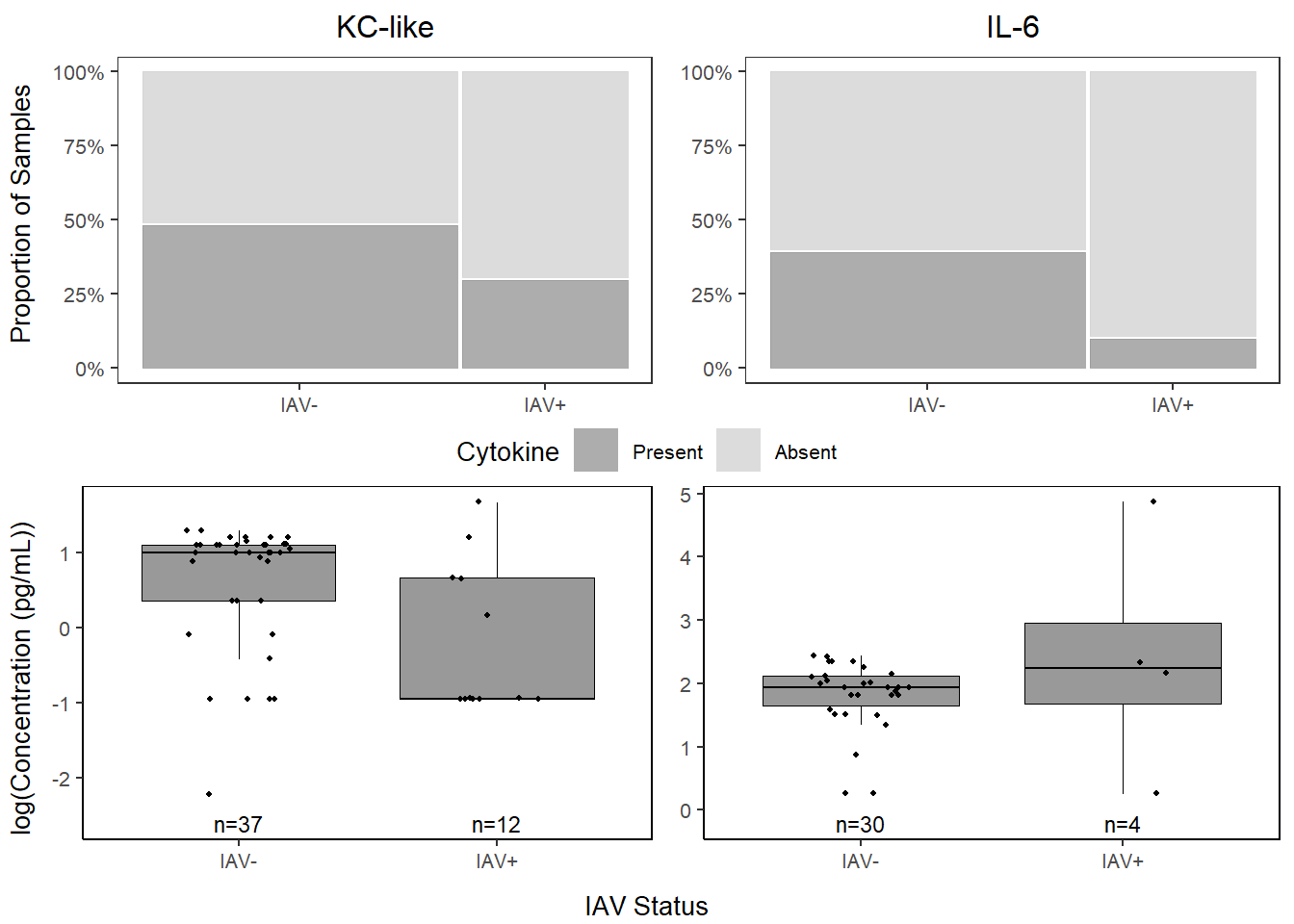

jpeg("Figures/cytoimportance.jpeg", width=7, height=8, units="in", res=300)
final_grid <- 
  grid.arrange(varimp_plot, cyto_grid, 
               ncol=1, heights=c(2,4)) 
grid.polygon(x=c(0, 0, 1, 1),
             y=c(0, 0.67, 0.67, 0),
             gp=gpar(fill=NA))
grid.rect(x=unit(0.49, "npc"), y = unit(0.95, "npc"),
          width=unit(0.94, "npc"), height=unit(0.06, "npc"), 
          gp=gpar(lwd=1.5, col="gray30", fill=NA))
dev.off()

## png 
##   2

6.6 Figures - All Cytokines

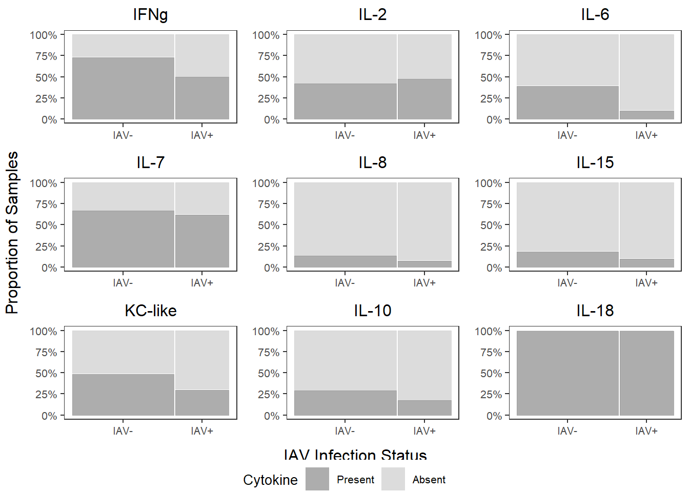
6.6.1 Cytokine Presence/Absence

kc_prop <-
  databin %>%
  ggplot(data=.) +
  geom_mosaic(aes(x=product(KC.like,iav), fill=KC.like)) +
  scale_fill_manual(values=c("Present"="gray60", "Absent"="lightgray"),
                    name="Cytokine") +
  scale_y_continuous(labels = scales::percent) +
  labs(title="KC-like") +
  theme_bw() +
  theme(panel.grid.major = element_blank(), 
        panel.grid.minor = element_blank(),
        axis.title.x = element_blank(),
        axis.title.y = element_blank(),
        legend.position="none",
        text = element_text(size=10),
        plot.title = element_text(hjust = 0.5))

il6_prop <-
  databin %>%
  ggplot(data=.) +
  geom_mosaic(aes(x=product(IL.6,iav), fill=IL.6)) +
  scale_fill_manual(values=c("Present"="gray60", "Absent"="lightgray"),
                    name="Cytokine") +
  scale_y_continuous(labels = scales::percent) +
  labs(title="IL-6") +
  theme_bw() +
  theme(panel.grid.major = element_blank(), 
        panel.grid.minor = element_blank(),
        axis.title.x = element_blank(),
        axis.title.y = element_blank(),
        legend.position="none",
        text = element_text(size=10),
        plot.title = element_text(hjust = 0.5))

ifng_prop <-
  databin %>%
  ggplot(data=.) +
  geom_mosaic(aes(x=product(IFNg,iav), fill=IFNg)) +
  scale_fill_manual(values=c("Present"="gray60", "Absent"="lightgray"),
                    name="Cytokine") +
  scale_y_continuous(labels = scales::percent) +
  labs(title="IFNg") +
  theme_bw() +
  theme(panel.grid.major = element_blank(), 
        panel.grid.minor = element_blank(),
        axis.title.x = element_blank(),
        axis.title.y = element_blank(),
        legend.position="none",
        text = element_text(size=10),
        plot.title = element_text(hjust = 0.5))

il2_prop <- 
  databin %>%
  ggplot(data=.) +
  geom_mosaic(aes(x=product(IL.2,iav), fill=IL.2)) +
  scale_fill_manual(values=c("Present"="gray60", "Absent"="lightgray")) +
  scale_y_continuous(labels = scales::percent) +
  labs(title="IL-2") +
  theme_bw() +
  theme(panel.grid.major = element_blank(), 
        panel.grid.minor = element_blank(),
        axis.title.x = element_blank(),
        axis.title.y = element_blank(),
        legend.position="none",
        text = element_text(size=10),
        plot.title = element_text(hjust = 0.5))

il7_prop <- 
  databin %>%
  ggplot(data=.) +
  geom_mosaic(aes(x=product(IL.7,iav), fill=IL.7)) +
  scale_fill_manual(values=c("Present"="gray60", "Absent"="lightgray")) +
  scale_y_continuous(labels = scales::percent) +
  labs(title="IL-7") +
  theme_bw() +
  theme(panel.grid.major = element_blank(), 
        panel.grid.minor = element_blank(),
        axis.title.x = element_blank(),
        axis.title.y = element_blank(),
        legend.position="none",
        text = element_text(size=10),
        plot.title = element_text(hjust = 0.5))

il8_prop <-
  databin %>%
  ggplot(data=.) +
  geom_mosaic(aes(x=product(IL.8,iav), fill=IL.8)) +
  scale_fill_manual(values=c("Present"="gray60", "Absent"="lightgray")) +
  scale_y_continuous(labels = scales::percent) +
  labs(title="IL-8") +
  theme_bw() +
  theme(panel.grid.major = element_blank(), 
        panel.grid.minor = element_blank(),
        axis.title.x = element_blank(),
        axis.title.y = element_blank(),
        legend.position="none",
        text = element_text(size=10),
        plot.title = element_text(hjust = 0.5))

il10_prop <- 
  databin %>%
  ggplot(data=.) +
  geom_mosaic(aes(x=product(IL.10,iav), fill=IL.10)) +
  scale_fill_manual(values=c("Present"="gray60", "Absent"="lightgray")) +
  scale_y_continuous(labels = scales::percent) +
  labs(title="IL-10") +
  theme_bw() +
  theme(panel.grid.major = element_blank(), 
        panel.grid.minor = element_blank(),
        axis.title.x = element_blank(),
        axis.title.y = element_blank(),
        legend.position="none",
        text = element_text(size=10),
        plot.title = element_text(hjust = 0.5))

il15_prop <- 
  databin %>%
  ggplot(data=.) +
  geom_mosaic(aes(x=product(IL.15,iav), fill=IL.15)) +
  scale_fill_manual(values=c("Present"="gray60", "Absent"="lightgray")) +
  scale_y_continuous(labels = scales::percent) +
  labs(title="IL-15") +
  theme_bw() +
  theme(panel.grid.major = element_blank(), 
        panel.grid.minor = element_blank(),
        axis.title.x = element_blank(),
        axis.title.y = element_blank(),
        legend.position="none",
        text = element_text(size=10),
        plot.title = element_text(hjust = 0.5))

il18_prop <-
  databin %>%
  ggplot(data=.) +
  geom_mosaic(aes(x=product(IL.18,iav), fill=IL.18)) +
  scale_fill_manual(values=c("Present"="gray60", "Absent"="lightgray")) +
  scale_y_continuous(labels = scales::percent) +
  labs(title="IL-18") +
  theme_bw() +
  theme(panel.grid.major = element_blank(), 
        panel.grid.minor = element_blank(),
        axis.title.x = element_blank(),
        axis.title.y = element_blank(),
        legend.position="none",
        text = element_text(size=10),
        plot.title = element_text(hjust = 0.5))

cyto_prop_grid <-
  grid.arrange(ifng_prop, il2_prop, il6_prop, 
               il7_prop, il8_prop, il15_prop, 
               kc_prop, il10_prop, il18_prop,
               left=textGrob("Proportion of Samples", rot=90),
               bottom=textGrob("IAV Infection Status"))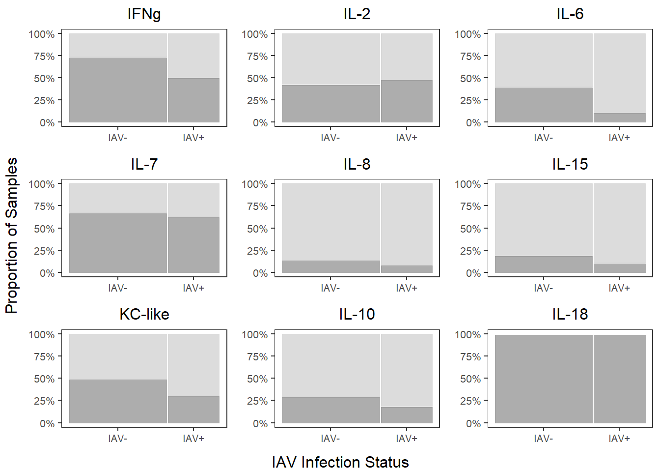

cyto_prop_grid <- 
  grid.arrange(cyto_prop_grid, cyto_leg, 
               ncol=1, 
               heights=c(9,0.5))

ggsave("Figures/cyto_prop_grid.jpeg", cyto_prop_grid, 
       width=8, height=8, units="in")

6.6.2 Cytokine Concentration - Log

kclike <- 
  data %>% 
  select(iav, KC.like) %>% 
  filter(!KC.like == 0) %>% 
  ggplot(., aes(x=iav, y=log(KC.like))) +
  geom_boxplot(color="black", fill="gray60", lwd=0.25,
               outliers=FALSE) +
  geom_point(size=0.75, position=position_jitter(width=0.2)) +
  labs(x=NULL, y=NULL, title="KC-like") +
  stat_n_text(size=4) +
  theme_classic() +
  theme(text = element_text(size=10),
        panel.border=element_rect(color="black", fill=NA, linewidth=0.5),
        plot.title = element_text(hjust=0.5))

il6 <-
  data %>% 
  select(iav, IL.6) %>% 
  filter(!IL.6 == 0) %>% 
  ggplot(., aes(x=iav, y=log(IL.6))) +
  geom_boxplot(color="black", fill="gray60", lwd=0.25,
               outliers=FALSE) +
  geom_point(size=0.75, position=position_jitter(width=0.2)) +
  labs(x=NULL, y=NULL, title="IL-6") +
  stat_n_text(size=4) +
  theme_classic() +
  theme(text = element_text(size=10),
        panel.border=element_rect(color="black", fill=NA, linewidth=0.5),
        plot.title = element_text(hjust=0.5))

ifng <-
  data %>% 
  select(iav, IFNg) %>% 
  filter(!IFNg == 0) %>% 
  ggplot(., aes(x=iav, y=log(IFNg))) +
  geom_boxplot(color="black", fill="gray60", lwd=0.25,
               outliers=FALSE) +
  geom_point(size=0.75, position=position_jitter(width=0.2)) +
  labs(x=NULL, y=NULL, title="IFNg") +
  stat_n_text(size=4) +
  theme_classic() +
  theme(text = element_text(size=10),
        panel.border=element_rect(color="black", fill=NA, linewidth=0.5),
        plot.title = element_text(hjust=0.5))

il2 <-
  data %>% 
  select(iav, IL.2) %>% 
  filter(!IL.2 == 0) %>% 
  ggplot(., aes(x=iav, y=log(IL.2))) +
  geom_boxplot(color="black", fill="gray60", lwd=0.25,
               outliers=FALSE) +
  geom_point(size=0.75, position=position_jitter(width=0.2)) +
  labs(x=NULL, y=NULL, title="IL-2") +
  stat_n_text(size=4) +
  theme_classic() +
  theme(text = element_text(size=10),
        panel.border=element_rect(color="black", fill=NA, linewidth=0.5),
        plot.title = element_text(hjust=0.5))

il7 <-
  data %>% 
  select(iav, IL.7) %>% 
  filter(!IL.7 == 0) %>% 
  ggplot(., aes(x=iav, y=log(IL.7))) +
  geom_boxplot(color="black", fill="gray60", lwd=0.25,
               outliers=FALSE) +
  geom_point(size=0.75, position=position_jitter(width=0.2)) +
  labs(x=NULL, y=NULL, title="IL-7") +
  stat_n_text(size=4) +
  theme_classic() +
  theme(text = element_text(size=10),
        panel.border=element_rect(color="black", fill=NA, linewidth=0.5),
        plot.title = element_text(hjust=0.5))

il8 <-
  data %>% 
  select(iav, IL.8) %>% 
  filter(!IL.8 == 0) %>% 
  ggplot(., aes(x=iav, y=log(IL.8))) +
  geom_boxplot(color="black", fill="gray60", lwd=0.25,
               outliers=FALSE) +
  geom_point(size=0.75, position=position_jitter(width=0.2)) +
  labs(x=NULL, y=NULL, title="IL-8") +
  stat_n_text(size=4) +
  theme_classic() +
  theme(text = element_text(size=10),
        panel.border=element_rect(color="black", fill=NA, linewidth=0.5),
        plot.title = element_text(hjust=0.5))

il10 <- 
  data %>% 
  select(iav, IL.10) %>% 
  filter(!IL.10 == 0) %>% 
  ggplot(., aes(x=iav, y=log(IL.10))) +
  geom_boxplot(color="black", fill="gray60", lwd=0.25,
               outliers=FALSE) +
  geom_point(size=0.75, position=position_jitter(width=0.2)) +
  labs(x=NULL, y=NULL, title="IL-10") +
  stat_n_text(size=4) +
  theme_classic() +
  theme(text = element_text(size=10),
        panel.border=element_rect(color="black", fill=NA, linewidth=0.5),
        plot.title = element_text(hjust=0.5))

il15 <-
  data %>% 
  select(iav, IL.15) %>% 
  filter(!IL.15 == 0) %>% 
  ggplot(., aes(x=iav, y=log(IL.15))) +
  geom_boxplot(color="black", fill="gray60", lwd=0.25,
               outliers=FALSE) +
  geom_point(size=0.75, position=position_jitter(width=0.2)) +
  labs(x=NULL, y=NULL, title="IL-15") +
  stat_n_text(size=4) +
  theme_classic() +
  theme(text = element_text(size=10),
        panel.border=element_rect(color="black", fill=NA, linewidth=0.5),
        plot.title = element_text(hjust=0.5))

il18 <- 
  data %>% 
  select(iav, IL.18) %>% 
  filter(!IL.18==0) %>% 
  ggplot(., aes(x=iav, y=log(IL.18))) +
  geom_boxplot(color="black", fill="gray60", lwd=0.25,
               outlier.size=0.75) +
  geom_point(size=0.75, position=position_jitter(width=0.2)) +
  labs(x=NULL, y=NULL, title="IL-18") +
  stat_n_text(size=4) +
  theme_classic() +
  theme(text=element_text(size=10),
         panel.border=element_rect(color="black", fill=NA, linewidth=0.5),
        plot.title = element_text(hjust=0.5))

cyto_conc_grid <-
  grid.arrange(ifng, il2, il6, 
               il7, il8, il15, 
               kclike, il10, il18, 
               ncol=3,
               left=textGrob("log(Cytokine Concentration (pg/mL))", rot=90),
               bottom=textGrob("IAV Infection Status"))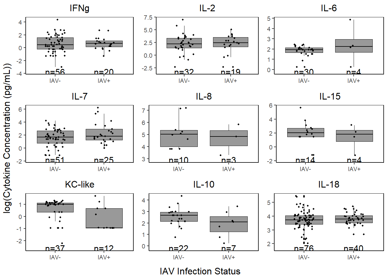

ggsave("Figures/supplemental_cyto_conc_grid.jpeg", cyto_conc_grid, 
       width=8, height=8, units="in")

6.7 Figures - Presentation

6.7.1 Presence/Absence

propdata <- 
  databin %>% 
  select(c(1:10, iav)) %>% 
  pivot_longer(2:10, names_to = "cytokine", values_to = "presence") %>% 
  mutate(presence = as.numeric(ifelse(presence == "Present", "1", "0"))) %>% 
  group_by(cytokine, iav) %>% 
  summarize(sum = sum(presence)) %>% 
  mutate(prop = ifelse(iav == "IAV+", sum/40, sum/76))

## `summarise()` has grouped output by 'cytokine'. You
## can override using the `.groups` argument.

prop_pres <-
  ggplot(propdata, aes(x = iav, y = prop, fill = iav)) +
  geom_col(position = "identity") +
  facet_wrap(~cytokine, ncol = 3) +
  scale_fill_manual(values = c("IAV-" = "#9d9d9d", "IAV+" = "#7FC1DB"),
                    name = "IAV Status") +
  scale_y_continuous(labels = scales::percent) +
  labs(x = NULL, y = "Proportion of Samples") +
  theme_bw() +
  theme(panel.grid = element_blank(),
        text = element_text(size = 16))

ggsave("Figures/cyto_prop_grid_pres.jpeg", prop_pres, 
       width=8, height=7, units="in")

6.7.2 Concentration

concdata <- 
  data %>% 
  select(c(1:10, iav)) %>% 
  pivot_longer(2:10, names_to = "cytokine", values_to = "concentration")


conc_pres <- 
  ggplot(concdata, aes(x = iav, y = log(concentration), fill = iav)) +
  geom_boxplot() +
  geom_point(size=0.75, position=position_jitter(width=0.2)) +
  facet_wrap(~cytokine, ncol = 3) +
  scale_fill_manual(values = c("IAV-" = "#9d9d9d", "IAV+" = "#7FC1DB"),
                    name = "IAV Status") +
  labs(x = NULL, y = "log(Concentration)") +
  theme_bw() +
  theme(panel.grid = element_blank(),
        text = element_text(size = 16))

ggsave("Figures/supplemental_cyto_conc_grid_pres.jpeg", conc_pres, 
       width=8, height=7, units="in")

## Warning: Removed 582 rows containing non-finite outside the
## scale range (`stat_boxplot()`).