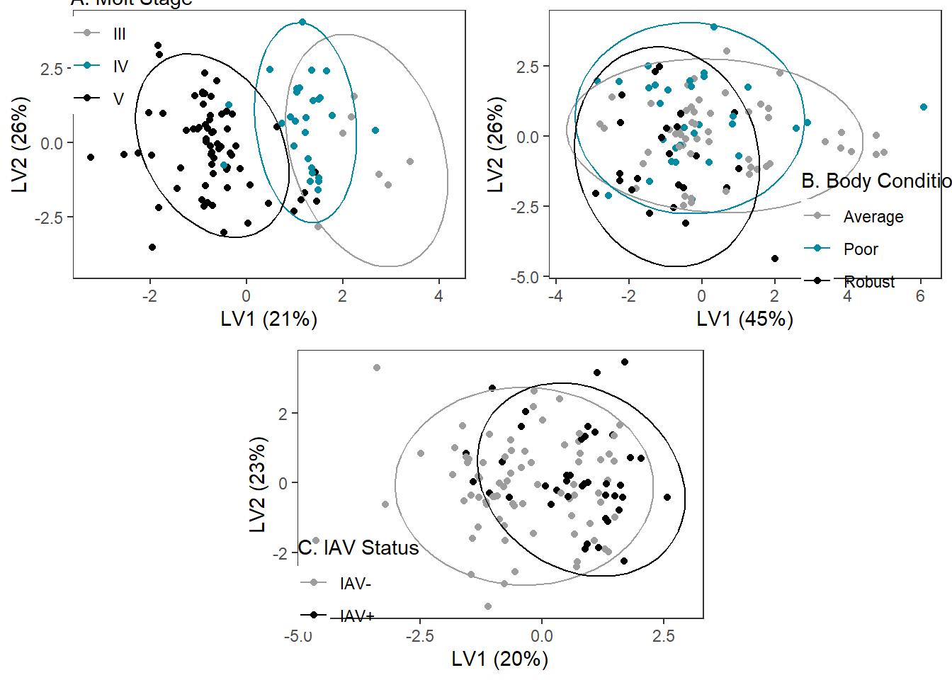
Molt Stage
molt_plsda <-
  mixOmics::plsda(data_molt[,2:10],
                  data_molt$molt.stage,
                  scale=TRUE)
molt_plsda_data <-
  data.frame(x = molt_plsda$variates$X[,1],
             y = molt_plsda$variates$X[,2],
             molt.stage = molt_plsda$Y)

# Set x and y axis labels based on prop of variation explained
labelx_molt <- paste("LV1 (",
                round(abs(molt_plsda$prop_expl_var$X[1]*100), digits=0),
                "%)",
                sep="")

labely_molt <- paste("LV2 (",
                round(abs(molt_plsda$prop_expl_var$X[2]*100), digits=0),
                "%)",
                sep="")

molt_plsda_ggplot <-
  ggplot(molt_plsda_data,
         aes(x=x, y=y, col=molt.stage)) +
  geom_point() +
  stat_ellipse() +
  labs(x=labelx_molt,
       y =labely_molt) +
  scale_color_manual("A. Molt Stage",
                     values=c("#9d9d9d","#008ba2", "black")) +
  theme_bw() +
  theme(panel.grid=element_blank(),
        legend.position = "inside",
        legend.position.inside = c(0.15, 0.85),
        legend.background = element_rect(fill=NA))
Body Condition
bc_plsda <-
  mixOmics::plsda(data_bc[,2:10],
                  data_bc$bc_bin,
                  scale=TRUE)

bc_plsda_data <-
  data.frame(x = bc_plsda$variates$X[,1],
             y = bc_plsda$variates$X[,2],
             bc = bc_plsda$Y)

# Set x and y axis labels based on prop of variation explained
labelx_bc <- paste("LV1 (",
                round(abs(bc_plsda$prop_expl_var$X[1]*100), digits=0),
                "%)",
                sep="")

labely_bc <- paste("LV2 (",
                round(abs(bc_plsda$prop_expl_var$X[2]*100), digits=0),
                "%)",
                sep="")

bc_plsda_ggplot <-
  ggplot(bc_plsda_data,
         aes(x=x, y=y, col=bc)) +
  geom_point() +
  stat_ellipse() +
  labs(x=labelx_bc,
       y = labely_bc) +
  scale_color_manual("B. Body Condition",
                     values=c("#9d9d9d","#008ba2", "black")) +
  theme_bw() +
  theme(panel.grid=element_blank(),
        legend.position = "inside",
        legend.position.inside = c(0.85, 0.17),
        legend.background = element_rect(fill=NA))
IAV
iav_plsda <-
  mixOmics::plsda(data_iav[,2:10],
                  data_iav$iav,
                  scale=TRUE)

iav_plsda_data <-
  data.frame(x = iav_plsda$variates$X[,1],
             y = iav_plsda$variates$X[,2],
             iav = iav_plsda$Y)

# Set x and y axis labels based on prop of variation explained
labelx_iav <- paste("LV1 (",
                round(abs(iav_plsda$prop_expl_var$X[1]*100), digits=0),
                "%)",
                sep="")

labely_iav <- paste("LV2 (",
                round(abs(iav_plsda$prop_expl_var$X[2]*100), digits=0),
                "%)",
                sep="")

iav_plsda_ggplot <-
  ggplot(iav_plsda_data,
         aes(x=x, y=y, col=iav)) +
  geom_point() +
  stat_ellipse() +
  labs(x=labelx_iav,
       y =labely_iav) +
  scale_color_manual("C. IAV Status",
                     values=c("#9d9d9d", "black")) +
  theme_bw() +
  theme(panel.grid=element_blank(),
        legend.position = "inside",
        legend.position.inside = c(0.15, 0.13),
        legend.background = element_rect(fill=NA))
Combine all plots
plsda_plots <- grid.arrange(molt_plsda_ggplot, bc_plsda_ggplot, iav_plsda_ggplot,
                            ncol=2, nrow=2,
                            layout_matrix=(rbind(c(1,1,2,2), c(NA,3,3,NA))))
ggsave("Figures/plsda_manuscript.jpeg", plsda_plots, width=10, height=8, units="in")