3 Exploratory

3.1 Libraries

library(mixOmics) # so tidyverse re-writes over select
library(tidyverse)
library(rstatix)

3.2 Initial Data Processing

3.2.1 Import data & merge

cyto <- 
  read.csv("Output Files/cleaned_cytokine_all.csv")
cytobin <-  
  read.csv("Output Files/cleaned_cytokine_bin_all.csv")

cyto_red <-
  read.csv("Output Files/cleaned_cytokine.csv")

meta <- 
  read.csv("Output Files/metadata_cyto.csv") %>% 
  mutate(iav=gsub("neg", "IAV-", iav),
         iav=gsub("pos", "IAV+", iav))

# Merge cytokine & meta data
data <- 
  merge(cyto, meta)

data_red <-
  merge(cyto_red, meta)

databin <- 
  merge(cytobin, meta) 

3.2.2 Ensure variables are correct format

data$iav <- as.factor(data$iav)
data$location <- as.factor(data$location)
data$year <- as.factor(data$year)
data$sex <- as.factor(data$sex)
data$molt.stage <- factor(data$molt.stage, levels=c("III", "IV", "V"), ordered=TRUE)
data$bc_bin <- factor(data$bc_bin, levels=c("Poor", "Average", "Robust"))
data$analysis.year <- ifelse(data$analysis.year=="2016", "1", 
                             ifelse(data$analysis.year=="2022", "2", "3"))
data$batch <- factor(data$batch, levels=c("1", "2", "3", "4"))

3.3 Descriptive Stats

3.3.1 Metadata Supplementary Table

supplmeta <- 
  data %>% 
  select(Sample, iav, iavser, location, year, sex, molt.stage, 
         bodcond, bc_bin, analysis.year) %>% 
  arrange(., year) %>% 
  mutate(bodcond=paste(round(bodcond, digits=2), " (", bc_bin, ")", sep=""),
         batch=analysis.year) %>% 
  select(-bc_bin, -analysis.year)
  
write.csv(supplmeta, "Output Files/supplemental_metadata.csv", row.names=FALSE)

3.3.2 Sample sizes across variables

table(supplmeta$iav)

## 
## IAV- IAV+ 
##   76   40

table(supplmeta$iavser)

## 
## neg pos 
##  86  30

table(supplmeta$location)

## 
## Great Point     Monomoy    Muskeget 
##          10          63          43

table(supplmeta$year)

## 
## 2014 2015 2016 2017 2018 2019 2020 2023 
##    5    7    9   25   17   17   10   26

table(supplmeta$sex)

## 
##  F  M 
## 62 51

table(supplmeta$molt.stage)

## 
## III  IV   V 
##   7  27  67

table(data$bc_bin)

## 
##    Poor Average  Robust 
##      31      52      25

table(data$analysis.year)

## 
##  1  2  3 
## 18 72 26

3.3.3 Cytokine detections per sample

num_samples <- apply(cyto[,2:14], 2, function(x) sum(x>0)) %>%
  data.frame() %>%
  mutate(perc=round((./116)*100, digits=2))
num_samples

##           .   perc
## GM.CSF    3   2.59
## IFNg     76  65.52
## IL.2     51  43.97
## IL.6     34  29.31
## IL.7     76  65.52
## IL.8     13  11.21
## IL.15    18  15.52
## IP.10     3   2.59
## KC.like  49  42.24
## IL.10    29  25.00
## IL.18   116 100.00
## MCP.1     1   0.86
## TNFa      2   1.72

3.3.4 Cytokine Ranges

cyto_pos <- 
  data %>% 
  filter(iav=="IAV+") %>% 
  select(1:14)

std.error <- function(x) sd(x)/sqrt(length(x))

pos_range <- 
  meta %>% 
  select(Sample, iav) %>% 
  filter(iav=="IAV+") %>% 
  merge(., cyto, by="Sample") %>% 
  pivot_longer(!c(iav, Sample), names_to="cytokine", values_to="concentration") %>% 
  filter(!concentration==0) %>% 
  group_by(cytokine) %>% 
  reframe(pos_sampsize=n(),
          mean=mean(concentration),
          se=std.error(concentration),
          median=median(concentration),
          min=min(concentration),
          max=max(concentration)) %>% 
  filter(!duplicated(.)) %>% 
  mutate(across(where(is.numeric), \(x) round(x, 2))) %>% 
  mutate(pos_meanse=paste(mean, "+", se),
         pos_medrange=paste(median, " (", min, " - ", max, ")", sep="")) %>% 
  select(cytokine, pos_sampsize, pos_meanse, pos_medrange)

neg_range <- 
  meta %>% 
  select(Sample, iav) %>% 
  filter(iav=="IAV-") %>% 
  merge(., cyto, by="Sample") %>% 
  pivot_longer(!c(iav, Sample), names_to="cytokine", values_to="concentration") %>% 
  filter(!concentration==0) %>% 
  group_by(cytokine) %>% 
  reframe(neg_sampsize=n(),
          mean=mean(concentration),
          se=std.error(concentration),
          median=median(concentration),
          min=min(concentration),
          max=max(concentration)) %>% 
  filter(!duplicated(.)) %>% 
  mutate(across(where(is.numeric), \(x) round(x, 2))) %>% 
  mutate(neg_meanse=paste(mean, "+", se),
         neg_medrange=paste(median, " (", min, " - ", max, ")", sep="")) %>% 
  select(cytokine, neg_sampsize, neg_meanse, neg_medrange)

table <- merge(neg_range, pos_range, by="cytokine", all.x=TRUE)
write.csv(table, "Output Files/manuscript_cytokinetable.csv", row.names=FALSE)

3.4 PCA

pca <- 
  prcomp(data_red[,2:10], center=TRUE, scale=TRUE)

pca_df <- 
  data.frame(
    x=pca$x[,1],
    y=pca$x[,2],
    molt.stage=data$molt.stage,
    year=factor(data$year),
    location=data$location,
    sex=data$sex,
    iav=data$iav,
    iavser=data$iavser,
    bc_bin=data$bc_bin,
    analysis.year=data$analysis.year,
    batch=data$batch
    )

pca_labelx <-
  paste("PC1 (", 
        round(abs(summary(pca)$importance[2,1]*100), digits=0),
        "%)",
        sep="")
pca_labely <-
  paste("PC2 (", 
        round(abs(summary(pca)$importance[2,2]*100), digits=0),
        "%)",
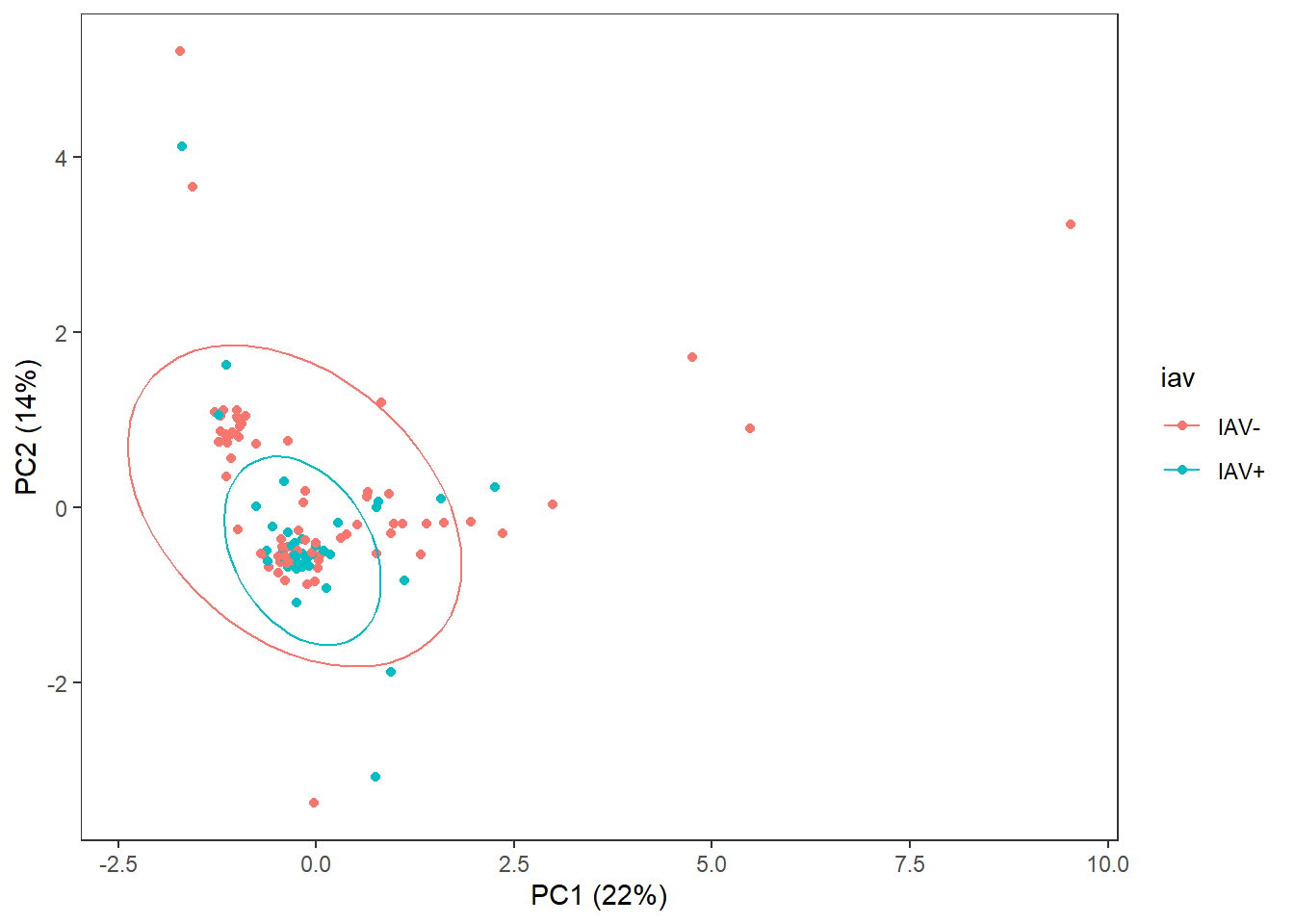
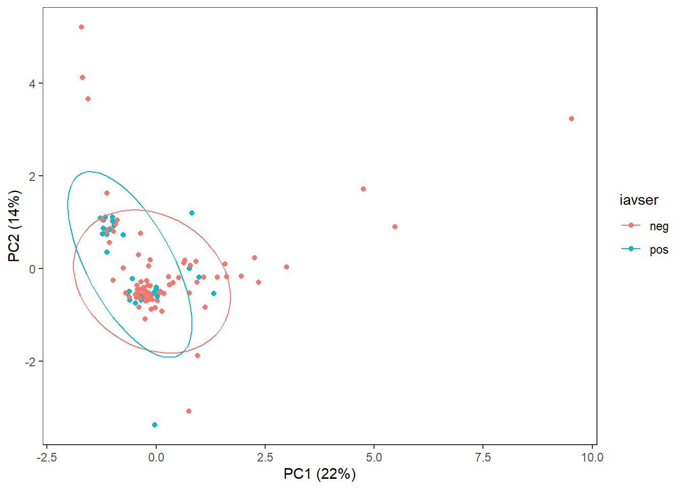
        sep="")

3.4.1 Molt Stage

ggplot(pca_df, 
       aes(x=x, 
           y=y,
           col=molt.stage)) +
  geom_point() +
  labs(x=pca_labelx,
       y = pca_labely) +
  scale_color_manual("Molt Stage",
                     values=c("#9d9d9d","#008ba2", "#000000")) +
  theme_bw() +
  theme(panel.grid=element_blank())

3.4.2 Year

ggplot(pca_df, 
       aes(x=x, 
           y=y,
           col=year)) +
  geom_point() +
  stat_ellipse() +
  labs(x=pca_labelx,
       y = pca_labely) +
  theme_bw() +
  theme(panel.grid=element_blank())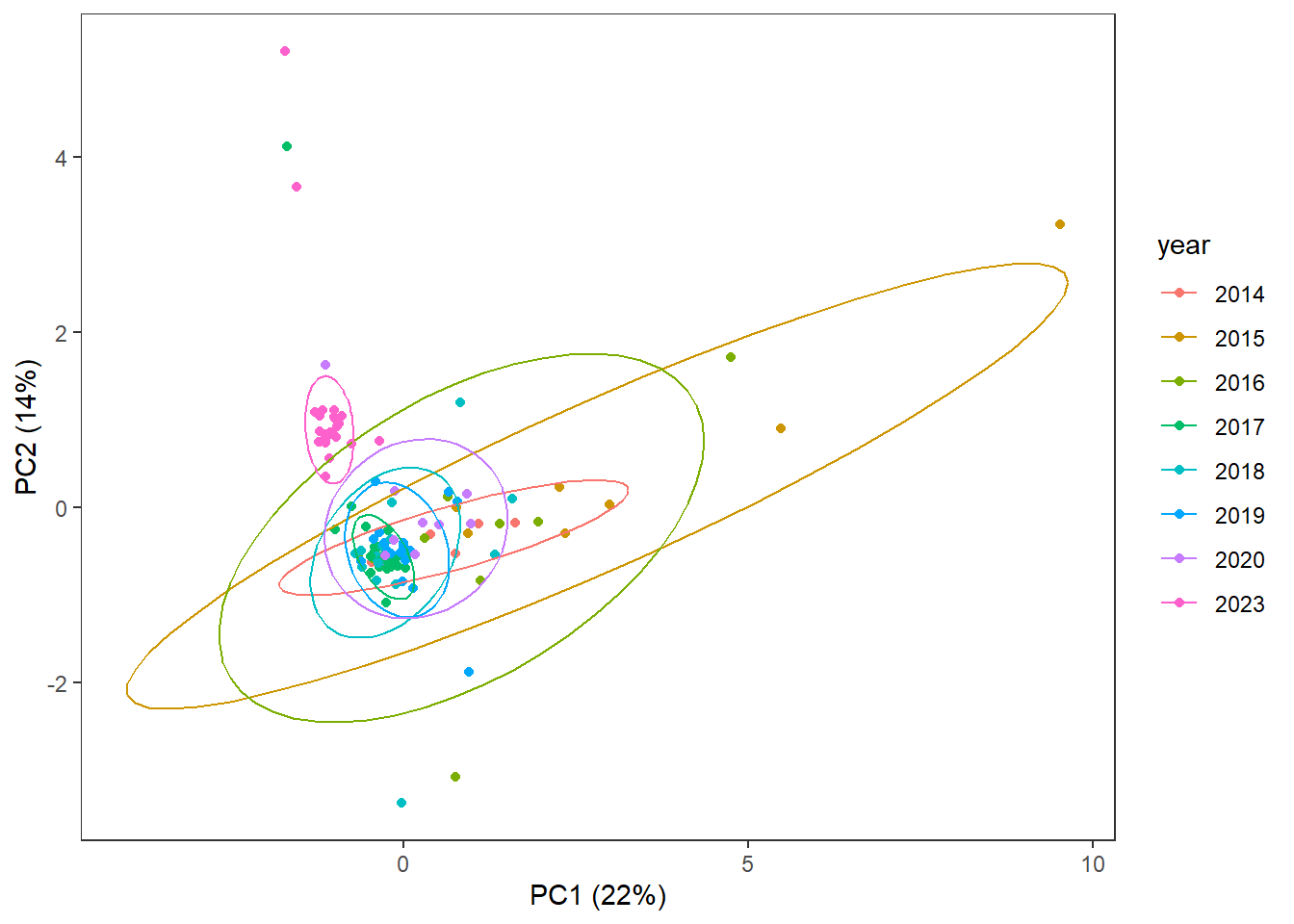

table(data$year, data$iav)

##       
##        IAV- IAV+
##   2014    5    0
##   2015    5    2
##   2016    7    2
##   2017    9   16
##   2018   12    5
##   2019    7   10
##   2020    6    4
##   2023   25    1

3.4.2.1 What’s up with year?

Similar # detections per sample as in other years (det.samp), and similar total cytokine concentrations per sample as in other years (sum.samp).

yeartab <-
  data.frame(table(data$year))
  
data %>% 
  select(Sample, 2:10, year) %>% 
  pivot_longer(!c(Sample, year), names_to="cytokine", values_to="concentration") %>%
  filter(!concentration==0) %>% 
  group_by(year) %>% 
  summarize(sum = sum(concentration),
            mean = mean(concentration),
            median = median(concentration),
            n.det = n(),
            n.cyto = length(unique(cytokine))) %>% 
  data.frame() %>% 
  merge(., yeartab, by.x="year", by.y="Var1") %>% 
  mutate(det.samp = n.det/Freq,
         sum.samp = sum/Freq)

##   year     sum      mean median n.det n.cyto Freq det.samp  sum.samp
## 1 2014  162.98  10.86533   5.45    15      6    5 3.000000  32.59600
## 2 2015 2142.65  97.39318  14.28    22      5    7 3.142857 306.09286
## 3 2016 2933.76 101.16414  10.44    29      7    9 3.222222 325.97333
## 4 2017  759.04  12.86508   4.76    59      7   25 2.360000  30.36160
## 5 2018  543.14  15.08722   6.54    36      7   17 2.117647  31.94941
## 6 2019  540.11  16.36697   2.14    33      4   17 1.941176  31.77118
## 7 2020  733.68  31.89913   4.86    23      6   10 2.300000  73.36800
## 8 2023 1913.16  18.04868   3.02   106      8   26 4.076923  73.58308

3.4.3 Analysis Year

Year that samples were analyzed, “batches”

analysisyear_plot <-
  ggplot(pca_df, 
       aes(x=x, 
           y=y,
           col=analysis.year)) +
  geom_point() +
  stat_ellipse() +
  scale_color_manual(values=c("black", "slategray3", "grey60"), 
                     name = "Batch") +
  labs(x = pca_labelx,
       y = pca_labely) +
  theme_bw() +
  theme(panel.grid = element_blank(),
        legend.position = "bottom")
analysisyear_plot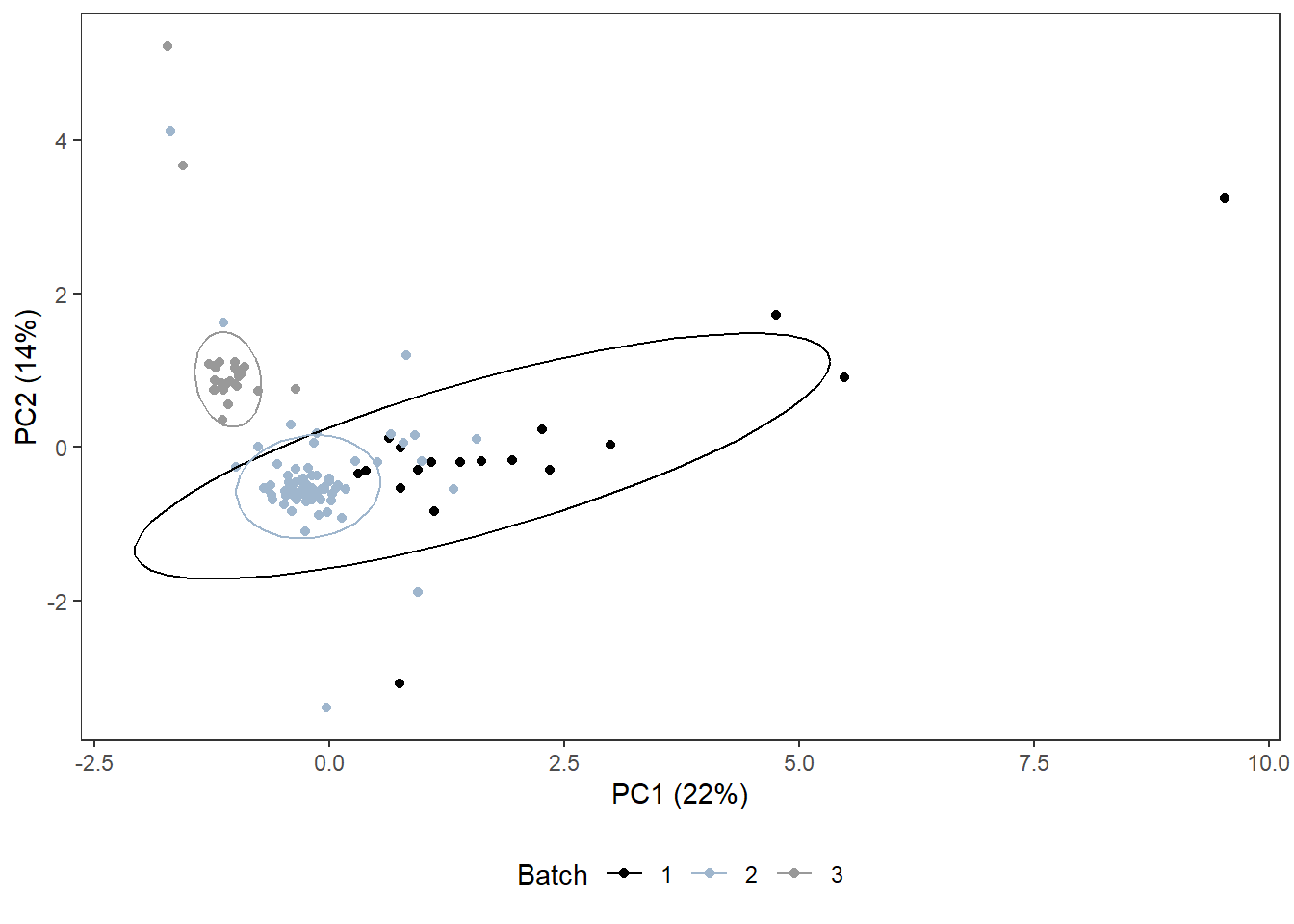

ggsave(filename="Figures/analysisyear_pca.jpeg", analysisyear_plot, 
       height=6, width=6, units="in")

biplot(pca)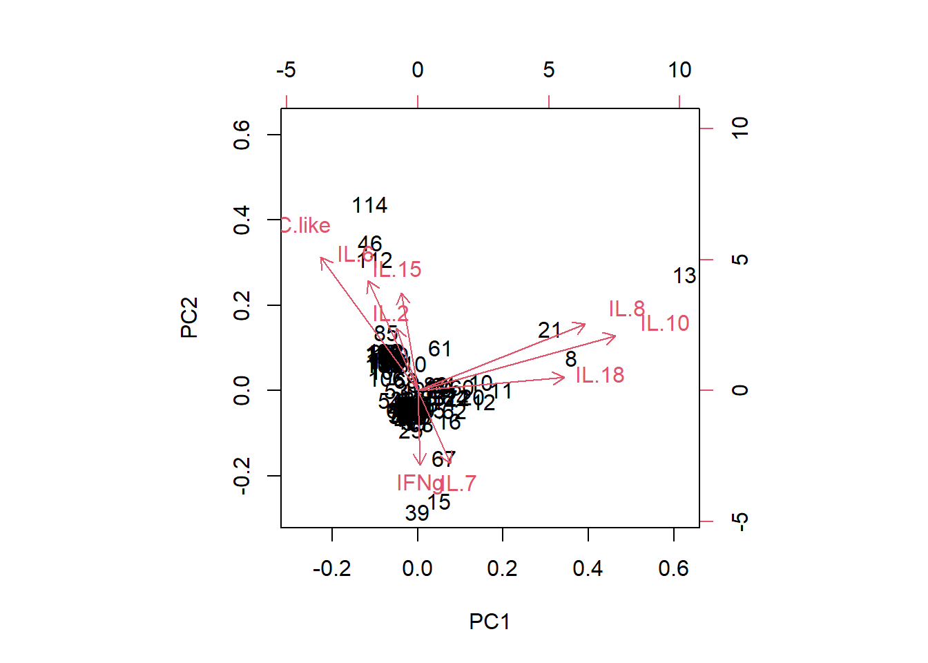

3.4.3.1 What’s up with analysis year?

Similar # detections per sample as in other years (det.samp), and similar total cytokine concentrations per sample as in other years (sum.samp).

analysisyeartab <-
  data.frame(table(data$analysis.year))
  
batchsummary <-
  data %>% 
  select(Sample, 2:14, analysis.year) %>% 
  pivot_longer(!c(Sample, analysis.year), names_to="cytokine", values_to="concentration") %>%
  filter(!concentration==0) %>% 
  group_by(analysis.year, cytokine) %>% 
  summarize(sum = sum(concentration),
            mean = mean(concentration),
            median = median(concentration),
            n.det = n(),
            n.cyto = length(unique(cytokine)),
            max = max(concentration)) %>% 
  data.frame() %>% 
  merge(., analysisyeartab, by.x="analysis.year", by.y="Var1") %>% 
  mutate(det.samp = n.det/Freq,
         sum.samp = sum/Freq)

## `summarise()` has grouped output by 'analysis.year'.
## You can override using the `.groups` argument.

# Mean cytokine concentration
ggplot(batchsummary, aes(x=cytokine, y=mean, fill=analysis.year)) +
  geom_col(position="dodge") +
  labs(y = "Mean Concentration") +
  scale_fill_manual(values=c("slategray", "slategray3", "slategray2"))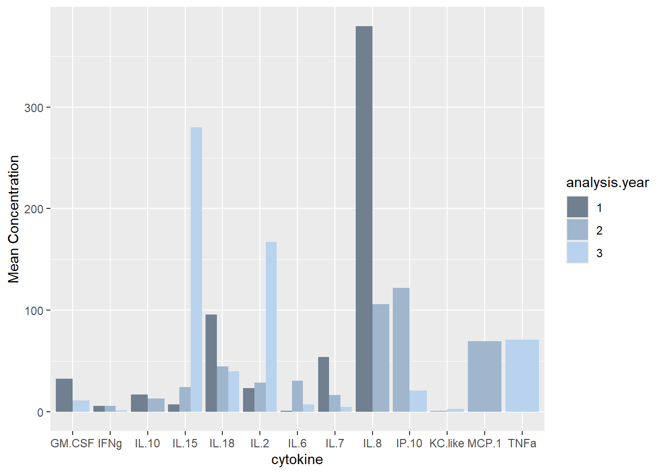

ggplot(batchsummary, aes(x=cytokine, y=log(mean), fill=analysis.year)) +
  geom_col(position="dodge") +
  labs(y = "Log Tranformed Mean Concentration") +
  scale_fill_manual(values=c("slategray", "slategray3", "slategray2"))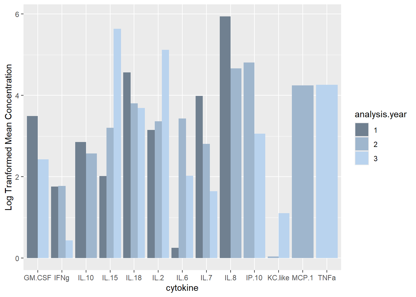

# Median cytokine concentration
ggplot(batchsummary, aes(x=cytokine, y=median, fill=analysis.year)) +
  geom_col(position="dodge") +
  labs(y = "Median Concentration") +
  scale_fill_manual(values=c("slategray", "slategray3", "slategray2"))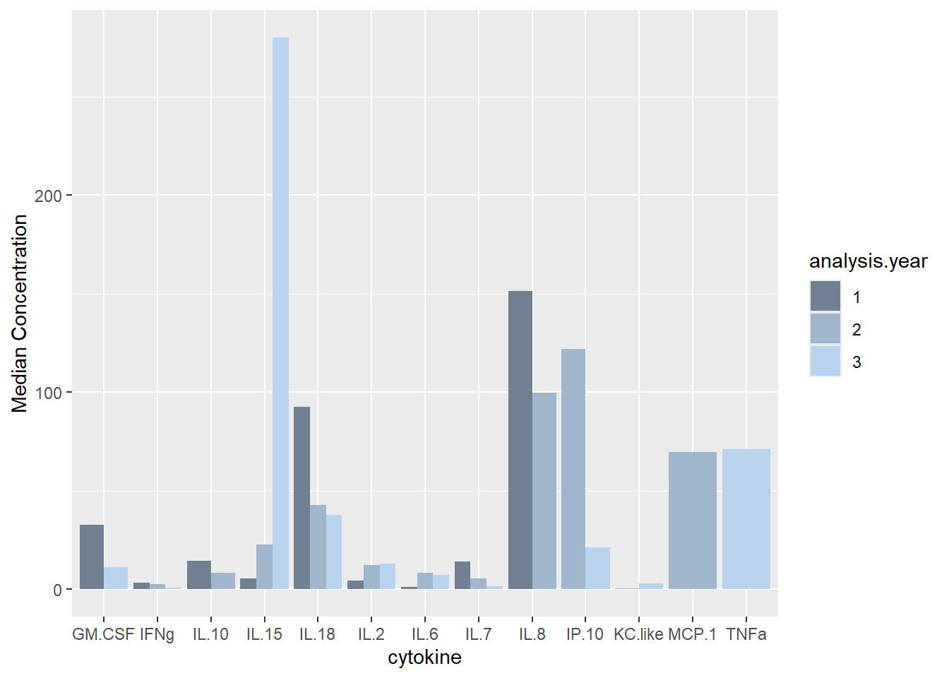

ggplot(batchsummary, aes(x=cytokine, y=log(median), fill=analysis.year)) +
  geom_col(position="dodge") +
  labs(y = "Log Transformed Median Concentration") +
  scale_fill_manual(values=c("slategray", "slategray3", "slategray2"))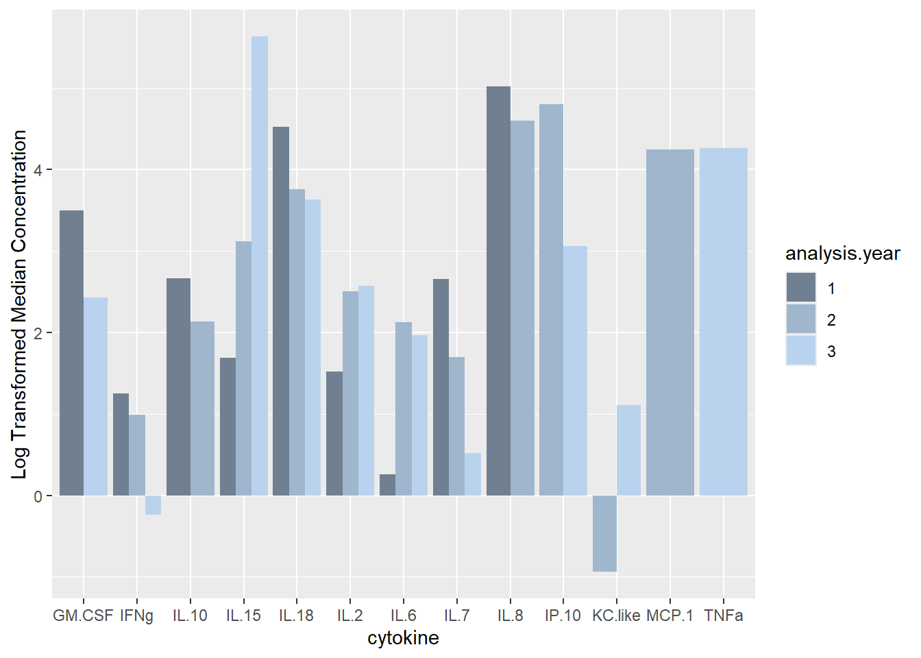

# Sum of cytokine concentrations, sum/sample
ggplot(batchsummary, aes(x=cytokine, y=log(sum), fill=analysis.year)) +
  geom_col(position="dodge") +
  labs(y = "Log Transformed Sum Concentration") +
  scale_fill_manual(values=c("slategray", "slategray3", "slategray2"))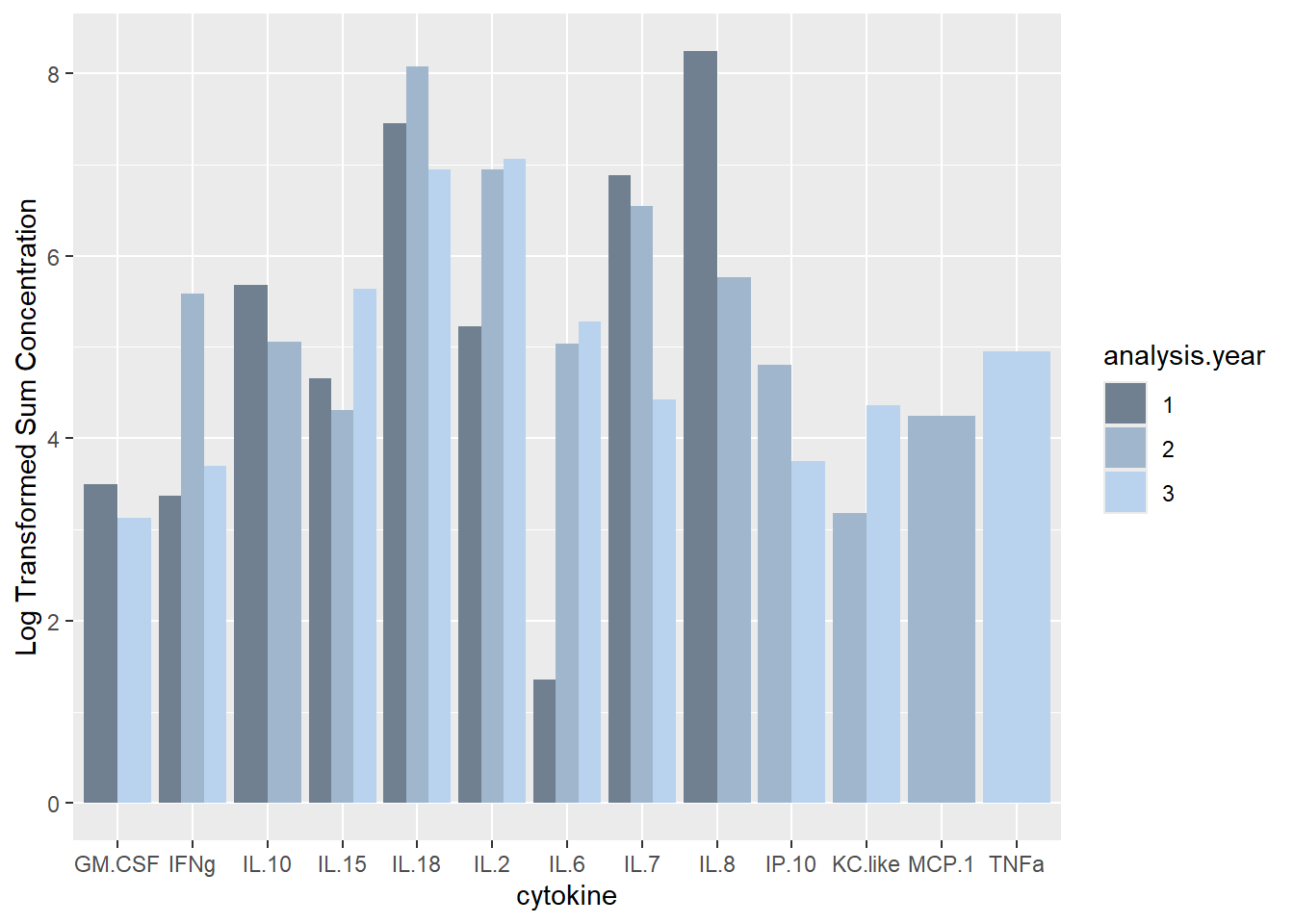

ggplot(batchsummary, aes(x=cytokine, y=log(sum.samp), fill=analysis.year)) +
  geom_col(position="dodge") +
  labs(y = "Log Transformed (Sum Concentration/Samples Analyzed)") +
  scale_fill_manual(values=c("slategray", "slategray3", "slategray2"))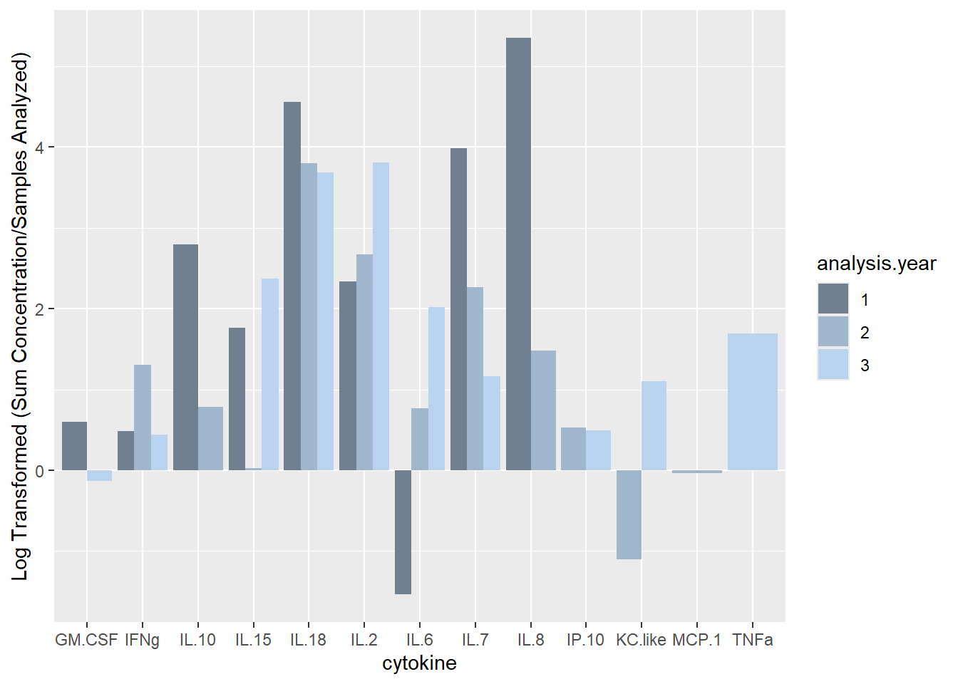

# Detections and proportion of samples with detections
ggplot(batchsummary, aes(x=cytokine, y=n.det, fill=analysis.year)) +
  geom_col(position="dodge") +
  labs(y = "Number of detections") +
  scale_fill_manual(values=c("slategray", "slategray3", "slategray2"))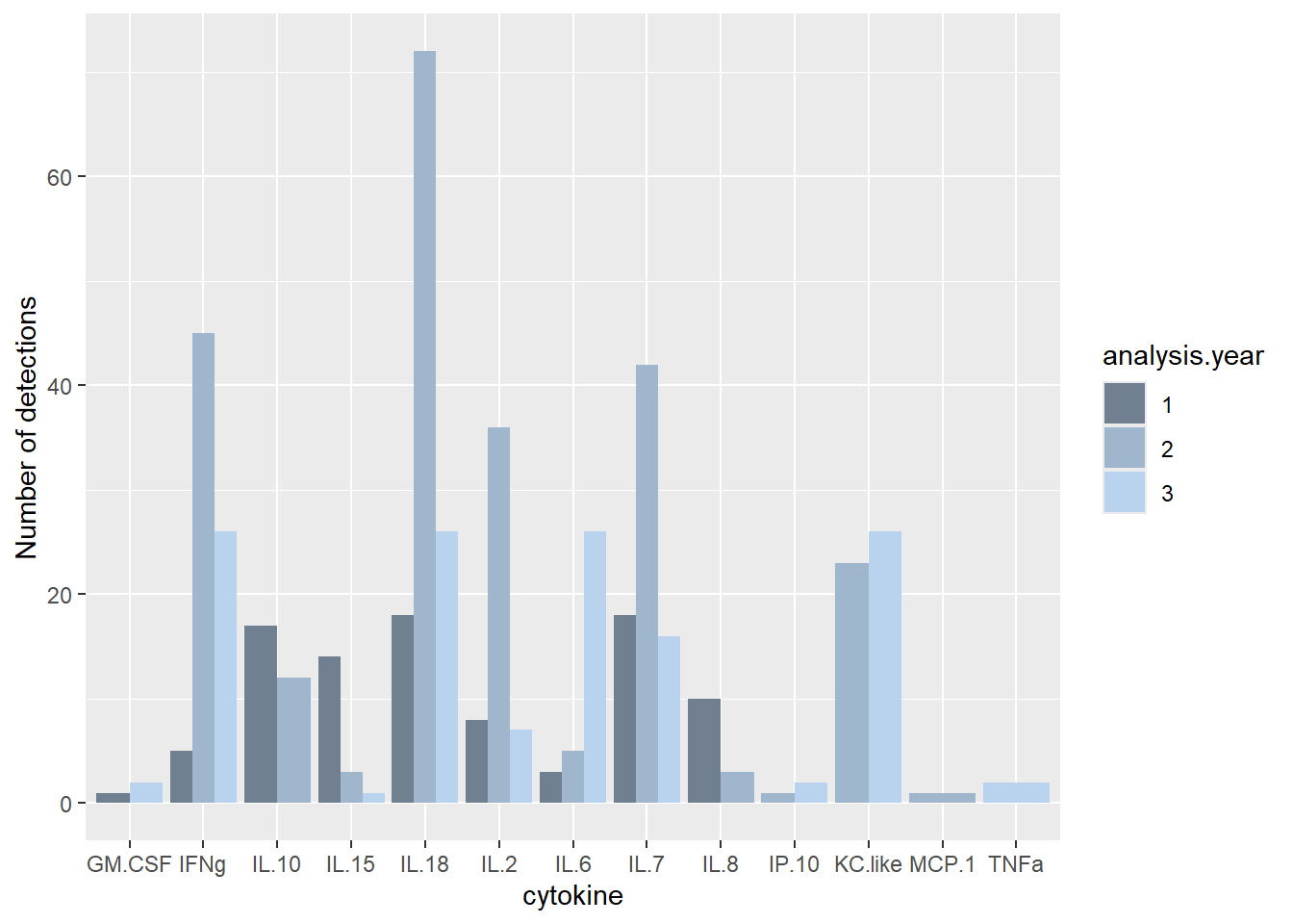

ggplot(batchsummary, aes(x=cytokine, y=det.samp, fill=analysis.year)) +
  geom_col(position="dodge") +
  labs(y = "Number of detections per Sample") +
  scale_fill_manual(values=c("slategray", "slategray3", "slategray2"))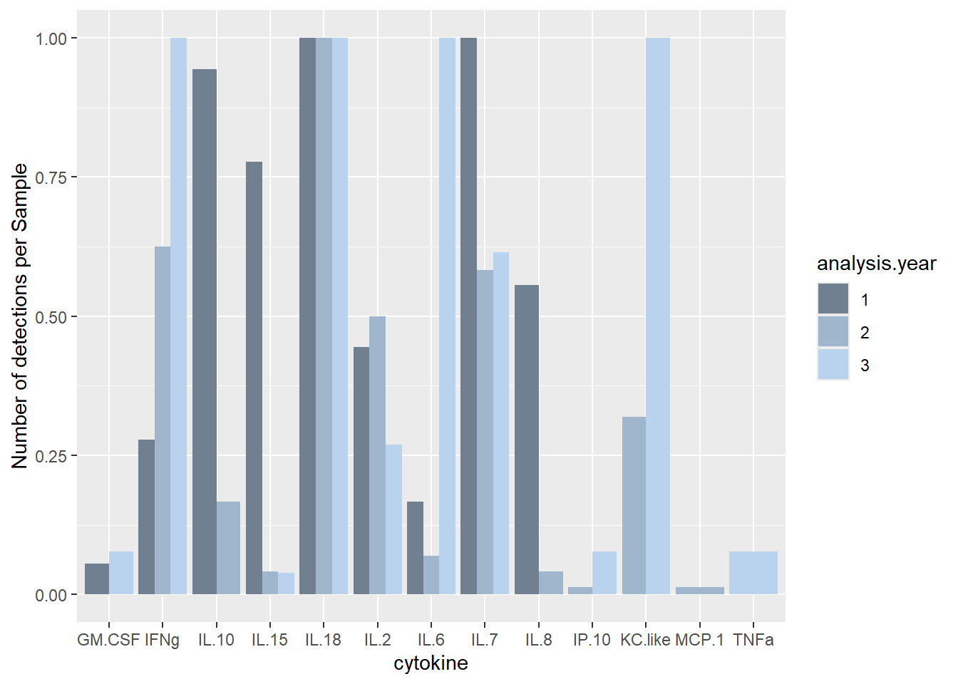

# Max detection of each cytokine
ggplot(batchsummary, aes(x=cytokine, y=max, fill=analysis.year)) +
  geom_col(position="dodge") +
  labs(y = "Max Detection") +
  scale_fill_manual(values=c("slategray", "slategray3", "slategray2"))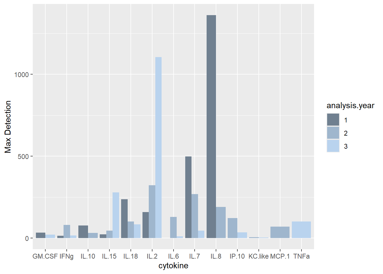

ggplot(batchsummary, aes(x=cytokine, y=log(max), fill=analysis.year)) +
  geom_col(position="dodge") +
  labs(y = "Log Transformed Max Detection") +
  scale_fill_manual(values=c("slategray", "slategray3", "slategray2"))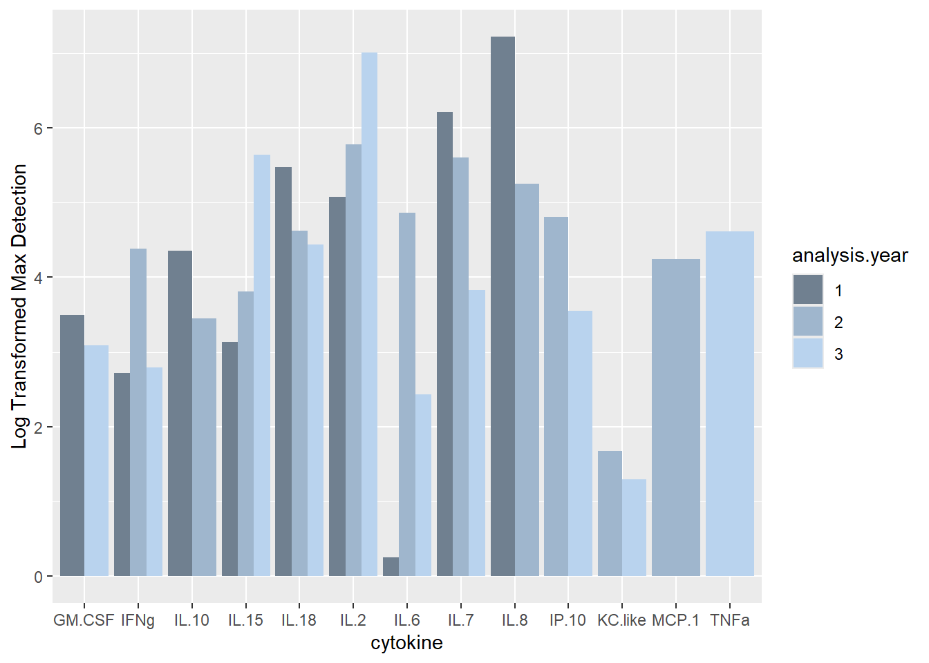

3.4.4 Batch

Batches that samples were analyzed in

ggplot(pca_df, 
       aes(x=x, 
           y=y,
           col=batch)) +
  geom_point() +
  stat_ellipse() +
  labs(x=pca_labelx,
       y = pca_labely) +
  theme_bw() +
  theme(panel.grid=element_blank())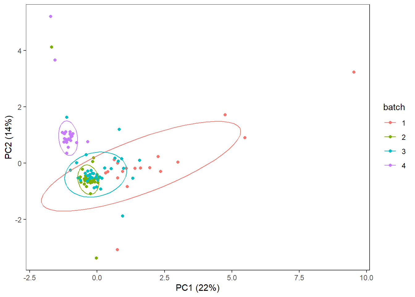

3.4.5 Location

ggplot(pca_df, 
       aes(x=x, 
           y=y,
           col=location)) +
  geom_point() +
  stat_ellipse() +
  labs(x=pca_labelx,
       y = pca_labely) +
  theme_bw() +
  theme(panel.grid=element_blank())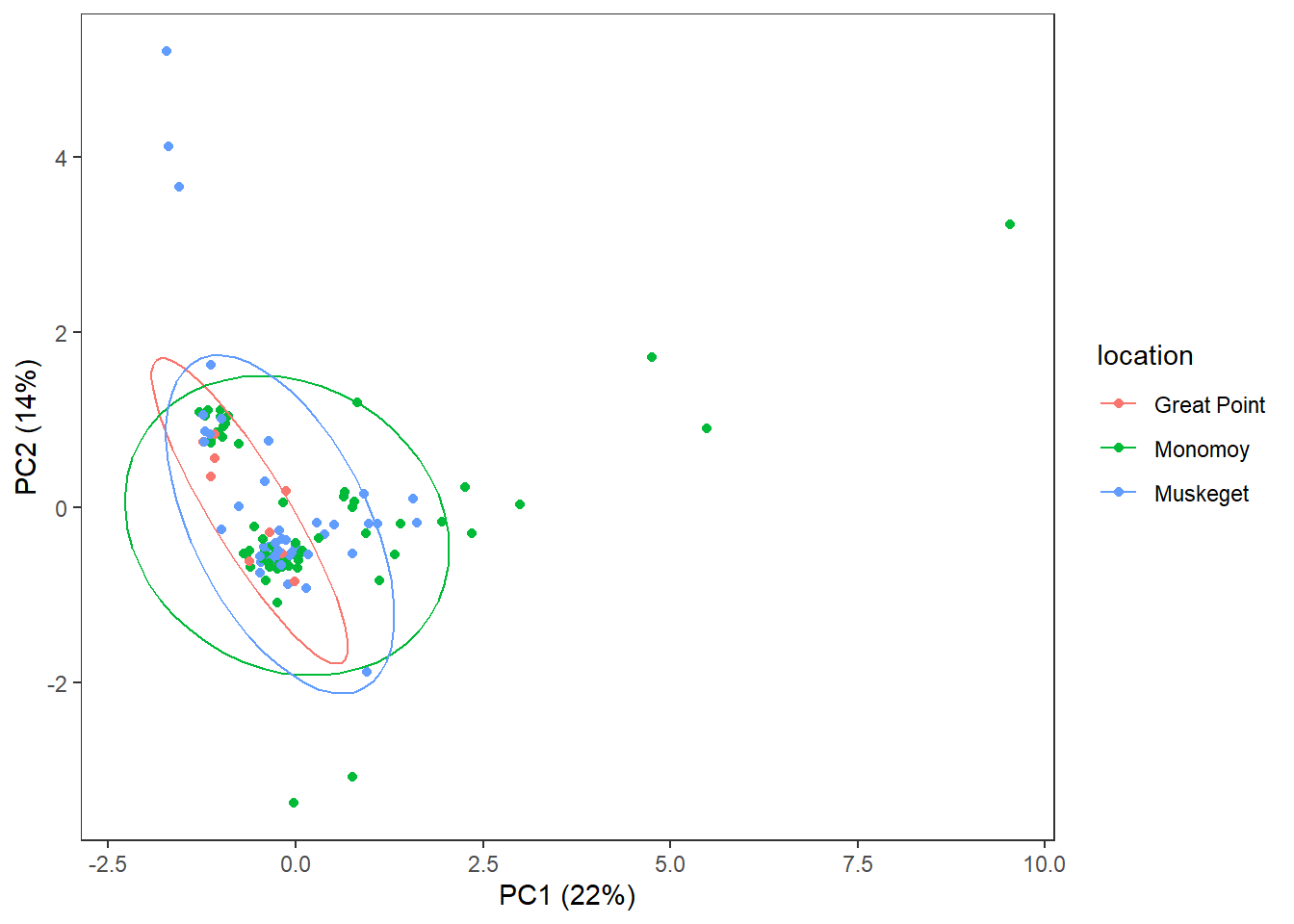

3.4.6 Sex

ggplot(pca_df, 
       aes(x=x, 
           y=y,
           col=sex)) +
  geom_point() +
  labs(x=pca_labelx,
       y = pca_labely) +
  theme_bw() +
  theme(panel.grid=element_blank())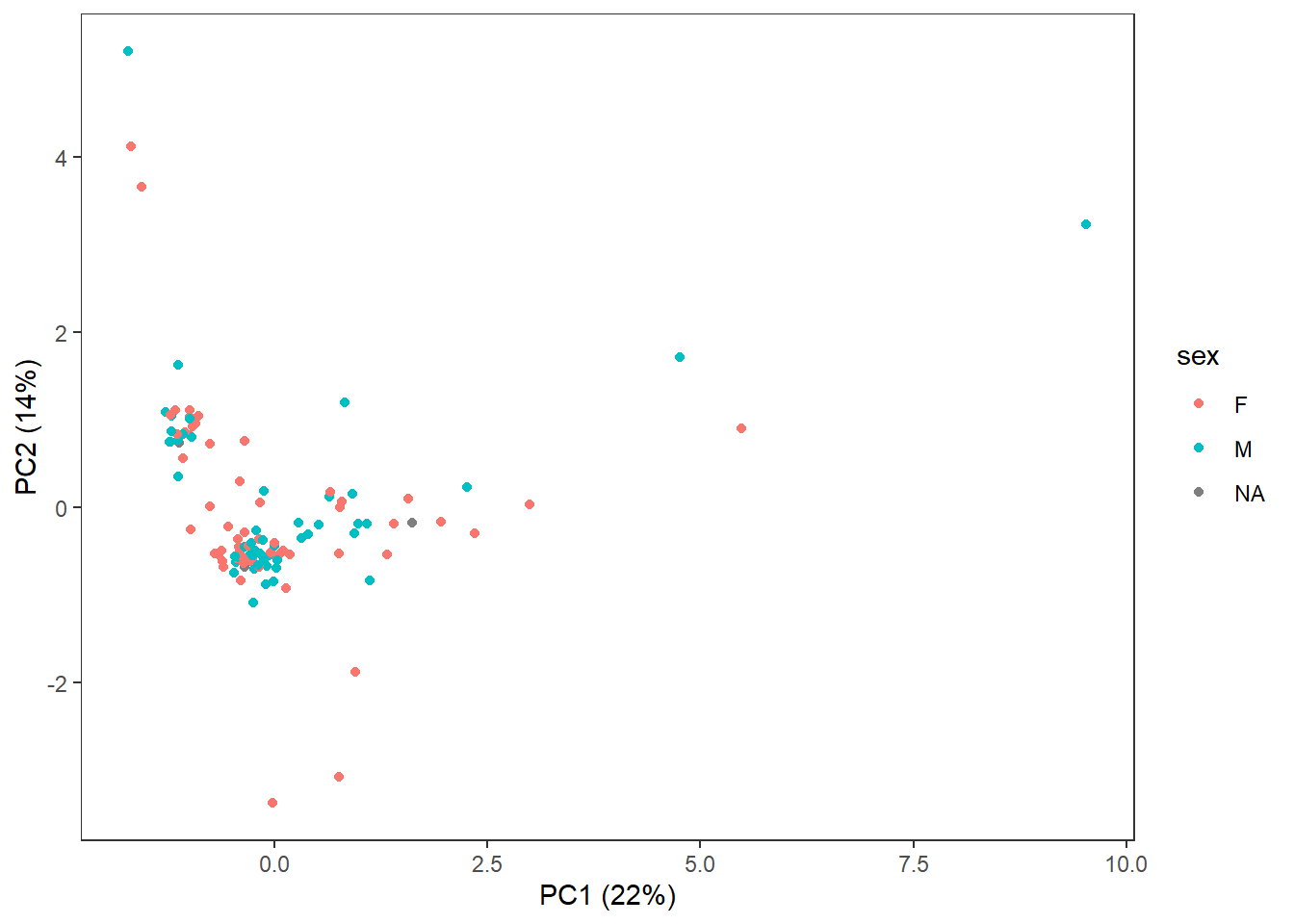

3.4.7 Body Condition

ggplot(pca_df, 
       aes(x=x, 
           y=y,
           col=bc_bin)) +
  geom_point() +
  labs(x=pca_labelx,
       y = pca_labely) +
  theme_bw() +
  theme(panel.grid=element_blank())

3.4.8 IAV

ggplot(pca_df, 
       aes(x=x, 
           y=y,
           col=iav)) +
  geom_point() +
  stat_ellipse() +
  labs(x=pca_labelx,
       y = pca_labely) +
  theme_bw() +
  theme(panel.grid=element_blank())

3.4.9 IAV Serology

ggplot(pca_df, 
       aes(x=x, 
           y=y,
           col=iavser)) +
  geom_point() +
  stat_ellipse() +
  labs(x=pca_labelx,
       y = pca_labely) +
  theme_bw() +
  theme(panel.grid=element_blank())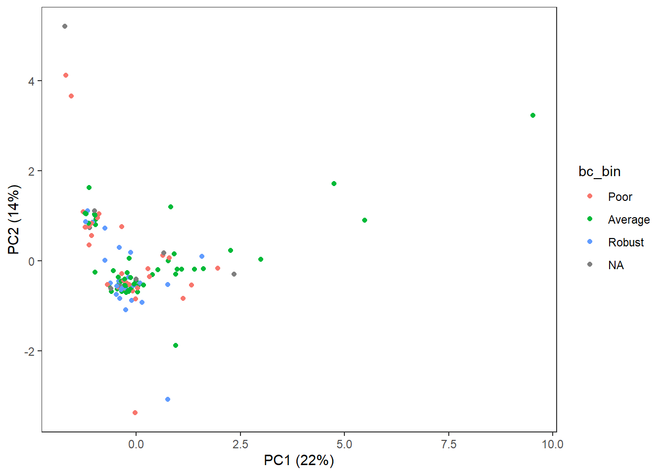

3.5 Is proportion of IAV+/IAV- similar across variables?

3.5.1 Analysis Year

tryCatch({
  chisq.test(table(data$analysis.year, data$iav))
}, warning = function(w) {
  fisher.test(table(data$analysis.year, data$iav))
})

## 
##  Pearson's Chi-squared test
## 
## data:  table(data$analysis.year, data$iav)
## X-squared = 18.361, df = 2, p-value = 0.000103

# Pairwise post-hoc
pairwise_fisher_test(table(data$analysis.year, data$iav), p.adjust.method="holm")

## # A tibble: 3 × 6
##   group1 group2     n         p     p.adj p.adj.signif
## * <chr>  <chr>  <int>     <dbl>     <dbl> <chr>       
## 1 1      2         90 0.0621    0.124     ns          
## 2 1      3         44 0.142     0.142     ns          
## 3 2      3         98 0.0000268 0.0000804 ****

data.frame(table(data$iav, data$analysis.year)) %>% 
  pivot_wider(names_from="Var1", values_from="Freq") %>% 
  mutate(proppos = (`IAV+`/(`IAV+` + `IAV-`))*100)

## # A tibble: 3 × 4
##   Var2  `IAV-` `IAV+` proppos
##   <fct>  <int>  <int>   <dbl>
## 1 1         14      4   22.2 
## 2 2         37     35   48.6 
## 3 3         25      1    3.85

3.5.2 Location

tryCatch({
  chisq.test(table(data$location, data$iav))
}, warning = function(w) {
  fisher.test(table(data$location, data$iav))
})

## 
##  Fisher's Exact Test for Count Data
## 
## data:  table(data$location, data$iav)
## p-value = 0.6994
## alternative hypothesis: two.sided

3.5.3 Molt Stage

tryCatch({
  chisq.test(table(data$molt.stage, data$iav))
}, warning = function(w) {
  fisher.test(table(data$molt.stage, data$iav))
})

## 
##  Fisher's Exact Test for Count Data
## 
## data:  table(data$molt.stage, data$iav)
## p-value = 0.04071
## alternative hypothesis: two.sided

# Pairwise post-hoc
pairwise_fisher_test(table(data$molt.stage, data$iav), p.adjust.method="holm")

## # A tibble: 3 × 6
##   group1 group2     n      p p.adj p.adj.signif
## * <chr>  <chr>  <int>  <dbl> <dbl> <chr>       
## 1 III    IV        34 0.681  0.681 ns          
## 2 III    V         74 0.0803 0.238 ns          
## 3 IV     V         94 0.0794 0.238 ns

data.frame(table(data$iav, data$molt.stage)) %>% 
  pivot_wider(names_from="Var1", values_from="Freq") %>% 
  mutate(proppos = (`IAV+`/(`IAV+` + `IAV-`))*100)

## # A tibble: 3 × 4
##   Var2  `IAV-` `IAV+` proppos
##   <fct>  <int>  <int>   <dbl>
## 1 III        3      4    57.1
## 2 IV        15     12    44.4
## 3 V         51     16    23.9

3.5.4 Body Condition

tryCatch({
  chisq.test(table(data$bc_bin, data$iav))
}, warning = function(w) {
  fisher.test(table(data$bc_bin, data$iav))
})

## 
##  Pearson's Chi-squared test
## 
## data:  table(data$bc_bin, data$iav)
## X-squared = 2.2554, df = 2, p-value = 0.3238